# Classification Recap and Linear Models
## Classification vs Regression
The goal of supervised learning is to make predictions using data. Supervised learning can be broken down into classification and regression problems.
### Regression
Regression involves predicting **continuous numerical values**, such as forecasting house prices or temperature. The problem of predicting house prices has no discrete solution space, which makes it a regression problem.
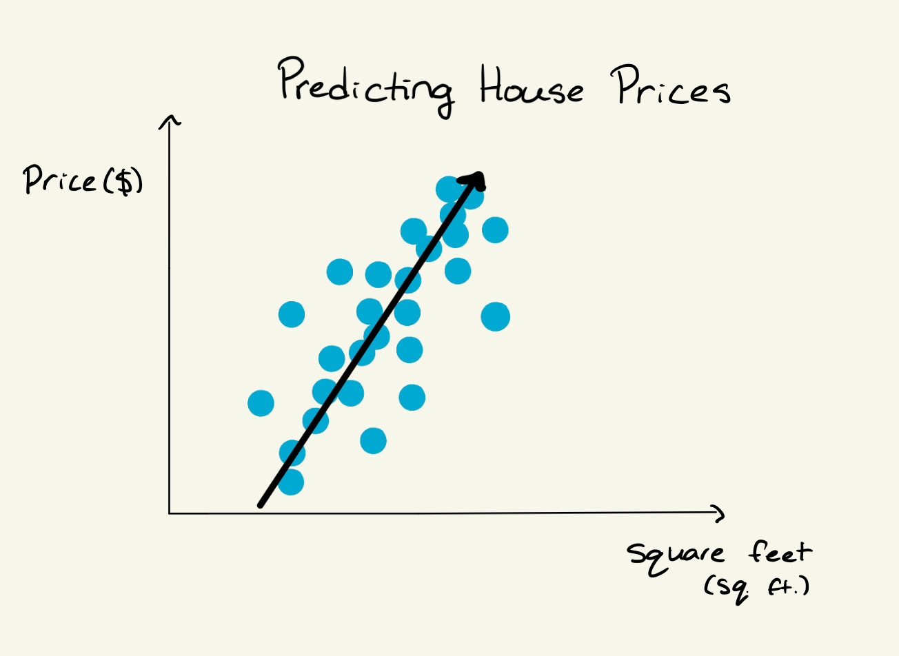 *A regression problem: predicting house prices from input features.*
### Classification
Classification is the task of predicting **discrete labels or categories**. The outcomes are distinct classes, such as classifying emails as spam or not spam.
Classification models learn from labeled data to find patterns that help predict class labels for unseen examples. Common real-world tasks include email spam detection, medical diagnosis, and sentiment analysis.
*A regression problem: predicting house prices from input features.*
### Classification
Classification is the task of predicting **discrete labels or categories**. The outcomes are distinct classes, such as classifying emails as spam or not spam.
Classification models learn from labeled data to find patterns that help predict class labels for unseen examples. Common real-world tasks include email spam detection, medical diagnosis, and sentiment analysis.
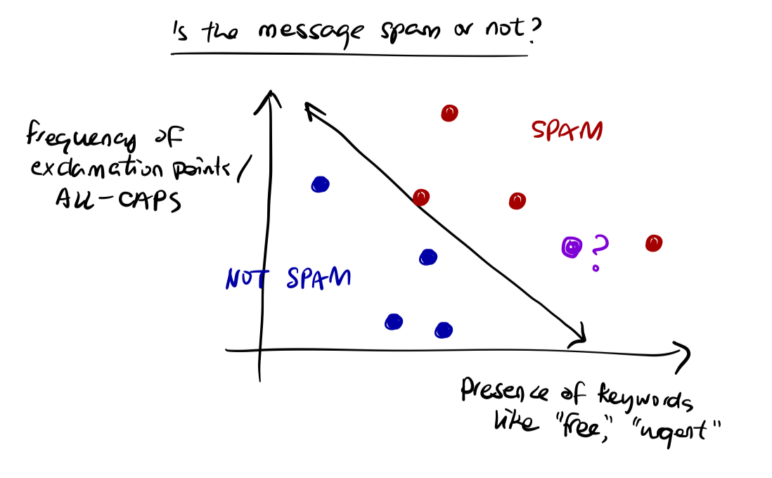 *A classification problem that seeks to answer "Is the message spam or not?" by classifying data into SPAM (+1) and NOT SPAM (-1).*
### Types of Classification
- **Binary Classification**: Predicting one of two classes (e.g., pass/fail, spam/ham, sick/healthy).
- **Multi-class Classification**: Predicting one of several possible classes (e.g., classifying digits 0 through 9, classifying animals into categories).
### Summary
| **Aspect** | **Classification** | **Regression** |
| -------------- | ---------------------------------------- | ----------------------------------------- |
| **Goal** | Predict discrete class labels | Predict continuous numeric values |
| **Output** | Categories (e.g., 0 or 1, A/B/C) | Real-valued numbers (e.g., price, weight) |
| **Examples** | Spam detection, disease diagnosis | House price prediction, temperature |
| **Evaluation** | Accuracy, Precision, Recall, F1-score | MSE, MAE, R-squared |
---
## Formal Setup
We aim to learn a model:
$$
f(\mathbf{x}; \theta): \mathbb{R}^d \to \{c_1, c_2, \dots, c_n\}
$$
that maps inputs to predicted labels.
- **Input**: $ \mathbf{x}_i \in \mathbb{R}^d $ is a feature vector (e.g., pixels in an image, GPA, attendance)
- **Label**: $ y_i \in \{c_1, c_2, \dots, c_n\} $ is the corresponding class label
- $ \theta $ are the **model parameters** (e.g., weights and biases) to be learned
- The training set consists of labeled examples: $ \{(\mathbf{x}_i, y_i)\}_{i=1}^N $
The learning objective is to adjust $ \theta $ so that the model's prediction $ f(\mathbf{x}_i; \theta) $ matches the true label $ y_i $ as closely as possible. At test time, we use the trained function to predict the label $ y $ for a new, unseen input $ \mathbf{x} $.
---
## Linear Models
A **linear model** assumes a linear relationship between the input features and the output. In classification, this means we assume the data is **linearly separable** -- there exists a hyperplane that can divide the input space into regions corresponding to different classes.
> A **hyperplane** is a flat, $ (d{-}1) $-dimensional subspace that separates a $ d $-dimensional space into two half-spaces.
The model computes a weighted sum:
$$
f(\mathbf{x}) = \mathbf{w}^\top \mathbf{x} + b
$$
where:
- $ \mathbf{w} \in \mathbb{R}^d $ is the **weight vector**
- $ \mathbf{x} \in \mathbb{R}^d $ is the **input feature vector**
- $ b \in \mathbb{R} $ is the **bias**
The hyperplane that splits the feature space is called the **decision boundary**.
### Binary Classification
For two classes $ y \in \{-1, +1\} $, predictions are made using:
$$
\hat{y} = \mathrm{sign}(\mathbf{w}^\top \mathbf{x} + b)
$$
where:
$$
\mathrm{sign}(z) =
\begin{cases}
+1, & z \ge 0 \\
-1, & z < 0
\end{cases}
$$
*A classification problem that seeks to answer "Is the message spam or not?" by classifying data into SPAM (+1) and NOT SPAM (-1).*
### Types of Classification
- **Binary Classification**: Predicting one of two classes (e.g., pass/fail, spam/ham, sick/healthy).
- **Multi-class Classification**: Predicting one of several possible classes (e.g., classifying digits 0 through 9, classifying animals into categories).
### Summary
| **Aspect** | **Classification** | **Regression** |
| -------------- | ---------------------------------------- | ----------------------------------------- |
| **Goal** | Predict discrete class labels | Predict continuous numeric values |
| **Output** | Categories (e.g., 0 or 1, A/B/C) | Real-valued numbers (e.g., price, weight) |
| **Examples** | Spam detection, disease diagnosis | House price prediction, temperature |
| **Evaluation** | Accuracy, Precision, Recall, F1-score | MSE, MAE, R-squared |
---
## Formal Setup
We aim to learn a model:
$$
f(\mathbf{x}; \theta): \mathbb{R}^d \to \{c_1, c_2, \dots, c_n\}
$$
that maps inputs to predicted labels.
- **Input**: $ \mathbf{x}_i \in \mathbb{R}^d $ is a feature vector (e.g., pixels in an image, GPA, attendance)
- **Label**: $ y_i \in \{c_1, c_2, \dots, c_n\} $ is the corresponding class label
- $ \theta $ are the **model parameters** (e.g., weights and biases) to be learned
- The training set consists of labeled examples: $ \{(\mathbf{x}_i, y_i)\}_{i=1}^N $
The learning objective is to adjust $ \theta $ so that the model's prediction $ f(\mathbf{x}_i; \theta) $ matches the true label $ y_i $ as closely as possible. At test time, we use the trained function to predict the label $ y $ for a new, unseen input $ \mathbf{x} $.
---
## Linear Models
A **linear model** assumes a linear relationship between the input features and the output. In classification, this means we assume the data is **linearly separable** -- there exists a hyperplane that can divide the input space into regions corresponding to different classes.
> A **hyperplane** is a flat, $ (d{-}1) $-dimensional subspace that separates a $ d $-dimensional space into two half-spaces.
The model computes a weighted sum:
$$
f(\mathbf{x}) = \mathbf{w}^\top \mathbf{x} + b
$$
where:
- $ \mathbf{w} \in \mathbb{R}^d $ is the **weight vector**
- $ \mathbf{x} \in \mathbb{R}^d $ is the **input feature vector**
- $ b \in \mathbb{R} $ is the **bias**
The hyperplane that splits the feature space is called the **decision boundary**.
### Binary Classification
For two classes $ y \in \{-1, +1\} $, predictions are made using:
$$
\hat{y} = \mathrm{sign}(\mathbf{w}^\top \mathbf{x} + b)
$$
where:
$$
\mathrm{sign}(z) =
\begin{cases}
+1, & z \ge 0 \\
-1, & z < 0
\end{cases}
$$
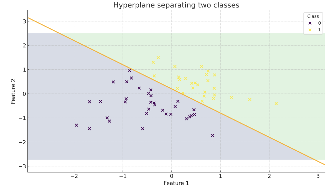 *A decision boundary separating two classes (represented by the orange line).*
### Multiclass Classification
For $ K $ classes, we train one linear model per class with parameters $ (\mathbf{w}_k, b_k) $. For each input $ \mathbf{x} $, we compute a score:
$$
s_k(\mathbf{x}) = \mathbf{w}_k^\top \mathbf{x} + b_k
$$
and predict the class with the highest score:
$$
\hat{y} = \underset{k}{\arg\max}\, s_k(\mathbf{x})
$$
*A decision boundary separating two classes (represented by the orange line).*
### Multiclass Classification
For $ K $ classes, we train one linear model per class with parameters $ (\mathbf{w}_k, b_k) $. For each input $ \mathbf{x} $, we compute a score:
$$
s_k(\mathbf{x}) = \mathbf{w}_k^\top \mathbf{x} + b_k
$$
and predict the class with the highest score:
$$
\hat{y} = \underset{k}{\arg\max}\, s_k(\mathbf{x})
$$
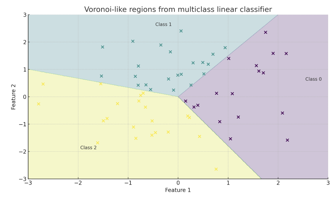 *A decision boundary separating $ K > 2 $ classes.*
> **Multiclass linear classifiers are not MLPs.** Even with $ K > 2 $ classes they still assume linear separability and produce straight (piecewise) decision boundaries. An MLP adds hidden layers and nonlinear activations, letting the boundary bend to fit non-linear patterns.
### The Bias Trick
The decision boundary is defined by $ \mathbf{w}^\top \mathbf{x} + b = 0 $. We can simplify notation by incorporating the bias into the weight vector. Append a 1 to the feature vector:
$$
\tilde{\mathbf{x}} = [\mathbf{x},\, 1], \quad \tilde{\mathbf{w}} = [\mathbf{w},\, b]
$$
Then the model becomes $ \tilde{\mathbf{w}}^\top \tilde{\mathbf{x}} $, eliminating the need to handle $ b $ separately.
### Learning Parameters
The parameters define the model's decision boundary:
- The **weight vector** $ \mathbf{w} $ controls the orientation of the hyperplane.
- The **bias** $ b $ shifts the boundary.
Our goal is to find values of $ \mathbf{w} $ and $ b $ that correctly classify the training examples. Different learning algorithms approach this differently:
- The **Perceptron algorithm** updates $ \mathbf{w} $ and $ b $ only when the model makes a mistake.
- **Logistic regression** defines a smoother notion of error using probabilities and uses **gradient descent** to gradually reduce that error.
---
## The Perceptron
The **Perceptron algorithm** is one of the earliest algorithms for training linear classifiers, developed at Cornell by Dr. Rosenblatt. In its basic form, it is a binary classifier that uses labels $ y \in \{-1, +1\} $ and updates the model only when it misclassifies a point.
### Forward Pass
The perceptron computes a prediction through the following steps:
1. **Input**: A feature vector $ \mathbf{x}_i = [x_i^0, x_i^1, \dots, x_i^d] $
2. **Weighted sum**: $ a_i = \mathbf{w}^\top \mathbf{x}_i + b $
3. **Step activation**: Apply the sign function to get $ \hat{y}_i = \mathrm{sign}(a_i) $
*A decision boundary separating $ K > 2 $ classes.*
> **Multiclass linear classifiers are not MLPs.** Even with $ K > 2 $ classes they still assume linear separability and produce straight (piecewise) decision boundaries. An MLP adds hidden layers and nonlinear activations, letting the boundary bend to fit non-linear patterns.
### The Bias Trick
The decision boundary is defined by $ \mathbf{w}^\top \mathbf{x} + b = 0 $. We can simplify notation by incorporating the bias into the weight vector. Append a 1 to the feature vector:
$$
\tilde{\mathbf{x}} = [\mathbf{x},\, 1], \quad \tilde{\mathbf{w}} = [\mathbf{w},\, b]
$$
Then the model becomes $ \tilde{\mathbf{w}}^\top \tilde{\mathbf{x}} $, eliminating the need to handle $ b $ separately.
### Learning Parameters
The parameters define the model's decision boundary:
- The **weight vector** $ \mathbf{w} $ controls the orientation of the hyperplane.
- The **bias** $ b $ shifts the boundary.
Our goal is to find values of $ \mathbf{w} $ and $ b $ that correctly classify the training examples. Different learning algorithms approach this differently:
- The **Perceptron algorithm** updates $ \mathbf{w} $ and $ b $ only when the model makes a mistake.
- **Logistic regression** defines a smoother notion of error using probabilities and uses **gradient descent** to gradually reduce that error.
---
## The Perceptron
The **Perceptron algorithm** is one of the earliest algorithms for training linear classifiers, developed at Cornell by Dr. Rosenblatt. In its basic form, it is a binary classifier that uses labels $ y \in \{-1, +1\} $ and updates the model only when it misclassifies a point.
### Forward Pass
The perceptron computes a prediction through the following steps:
1. **Input**: A feature vector $ \mathbf{x}_i = [x_i^0, x_i^1, \dots, x_i^d] $
2. **Weighted sum**: $ a_i = \mathbf{w}^\top \mathbf{x}_i + b $
3. **Step activation**: Apply the sign function to get $ \hat{y}_i = \mathrm{sign}(a_i) $
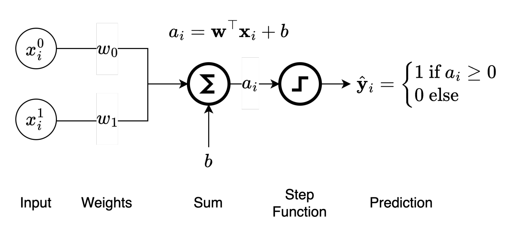 *Perceptron prediction diagram -- the forward pass for computing the predicted label $ \hat{y}_i $ from input $ \mathbf{x}_i $.*
*[Image credit: Kilian Q. Weinberger and Jennifer J. Sun via [CS 4782](https://www.cs.cornell.edu/courses/cs4782/2025sp/slides/pdf/week1_2_slides.pdf)]*
### Perceptron Update Rule
Given training data $ \{(\mathbf{x}_i, y_i)\}_{i=1}^N $, the Perceptron algorithm proceeds as follows:
1. Initialize $ \mathbf{w} = \mathbf{0} $, $ b = 0 $
2. For each example $ (\mathbf{x}_i, y_i) $:
- Compute prediction: $ \hat{y}_i = \mathrm{sign}(\mathbf{w}^\top \mathbf{x}_i + b) $
- If misclassified (i.e., $ y_i (\mathbf{w}^\top \mathbf{x}_i + b) \le 0 $), update:
$$
\mathbf{w} \leftarrow \mathbf{w} + y_i \mathbf{x}_i, \qquad b \leftarrow b + y_i
$$
3. Terminate when the perceptron no longer makes mistakes (assuming data is linearly separable).
*Perceptron prediction diagram -- the forward pass for computing the predicted label $ \hat{y}_i $ from input $ \mathbf{x}_i $.*
*[Image credit: Kilian Q. Weinberger and Jennifer J. Sun via [CS 4782](https://www.cs.cornell.edu/courses/cs4782/2025sp/slides/pdf/week1_2_slides.pdf)]*
### Perceptron Update Rule
Given training data $ \{(\mathbf{x}_i, y_i)\}_{i=1}^N $, the Perceptron algorithm proceeds as follows:
1. Initialize $ \mathbf{w} = \mathbf{0} $, $ b = 0 $
2. For each example $ (\mathbf{x}_i, y_i) $:
- Compute prediction: $ \hat{y}_i = \mathrm{sign}(\mathbf{w}^\top \mathbf{x}_i + b) $
- If misclassified (i.e., $ y_i (\mathbf{w}^\top \mathbf{x}_i + b) \le 0 $), update:
$$
\mathbf{w} \leftarrow \mathbf{w} + y_i \mathbf{x}_i, \qquad b \leftarrow b + y_i
$$
3. Terminate when the perceptron no longer makes mistakes (assuming data is linearly separable).
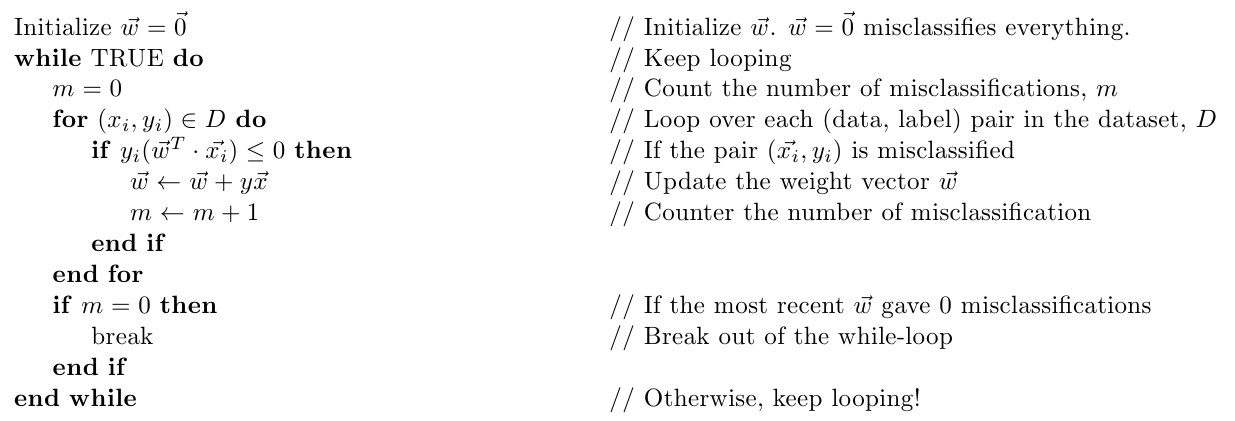 *The Perceptron algorithm.*
*[Image credit: Kilian Q. Weinberger and Jennifer J. Sun via [CS 4782](https://www.cs.cornell.edu/courses/cs4782/2025sp/slides/pdf/week1_2_slides.pdf)]*
### Intuition
Only examples that are misclassified trigger updates. The update pushes the decision boundary in a direction that makes the current example more likely to be classified correctly in the future. This nudging gradually adjusts the hyperplane to better separate the two classes.
The perceptron is particularly dependent on the assumption of linear separability due to its termination condition. When the data are not perfectly separable, the perceptron can cycle indefinitely without converging.
---
## Logistic Regression
The Perceptron makes **hard decisions** -- it only tells us which side of the hyperplane an input lies on, and only updates when it is wrong. In many problems, we would like to:
- Know how **confident** the model is in a prediction
- Update the model **gradually** even when it is close to correct
- Handle **non-separable** data more gracefully
### From Linear Scores to Probabilities
Like the perceptron, logistic regression starts with a linear score:
$$
a = \mathbf{w}^\top \mathbf{x} + b
$$
But instead of applying the step function, it passes the score through the **sigmoid function**:
$$
\sigma(a) = \frac{1}{1 + e^{-a}} \in (0, 1)
$$
This gives a prediction:
$$
\hat{y} = \sigma(\mathbf{w}^\top \mathbf{x} + b)
$$
which we interpret as the probability that $ \mathbf{x} $ belongs to the positive class, i.e., $ P(y = 1 \mid \mathbf{x}) $.
### Why Sigmoid?
- It "squashes" real values to a range between 0 and 1, interpretable as a probability.
- Values near 0.5 indicate uncertainty; values near 0 or 1 indicate high confidence.
- It is smooth and differentiable, which is important for gradient-based optimization.
- The decision boundary is at $ \hat{y} = 0.5 $, which corresponds to $ \mathbf{w}^\top \mathbf{x} + b = 0 $.
*The Perceptron algorithm.*
*[Image credit: Kilian Q. Weinberger and Jennifer J. Sun via [CS 4782](https://www.cs.cornell.edu/courses/cs4782/2025sp/slides/pdf/week1_2_slides.pdf)]*
### Intuition
Only examples that are misclassified trigger updates. The update pushes the decision boundary in a direction that makes the current example more likely to be classified correctly in the future. This nudging gradually adjusts the hyperplane to better separate the two classes.
The perceptron is particularly dependent on the assumption of linear separability due to its termination condition. When the data are not perfectly separable, the perceptron can cycle indefinitely without converging.
---
## Logistic Regression
The Perceptron makes **hard decisions** -- it only tells us which side of the hyperplane an input lies on, and only updates when it is wrong. In many problems, we would like to:
- Know how **confident** the model is in a prediction
- Update the model **gradually** even when it is close to correct
- Handle **non-separable** data more gracefully
### From Linear Scores to Probabilities
Like the perceptron, logistic regression starts with a linear score:
$$
a = \mathbf{w}^\top \mathbf{x} + b
$$
But instead of applying the step function, it passes the score through the **sigmoid function**:
$$
\sigma(a) = \frac{1}{1 + e^{-a}} \in (0, 1)
$$
This gives a prediction:
$$
\hat{y} = \sigma(\mathbf{w}^\top \mathbf{x} + b)
$$
which we interpret as the probability that $ \mathbf{x} $ belongs to the positive class, i.e., $ P(y = 1 \mid \mathbf{x}) $.
### Why Sigmoid?
- It "squashes" real values to a range between 0 and 1, interpretable as a probability.
- Values near 0.5 indicate uncertainty; values near 0 or 1 indicate high confidence.
- It is smooth and differentiable, which is important for gradient-based optimization.
- The decision boundary is at $ \hat{y} = 0.5 $, which corresponds to $ \mathbf{w}^\top \mathbf{x} + b = 0 $.
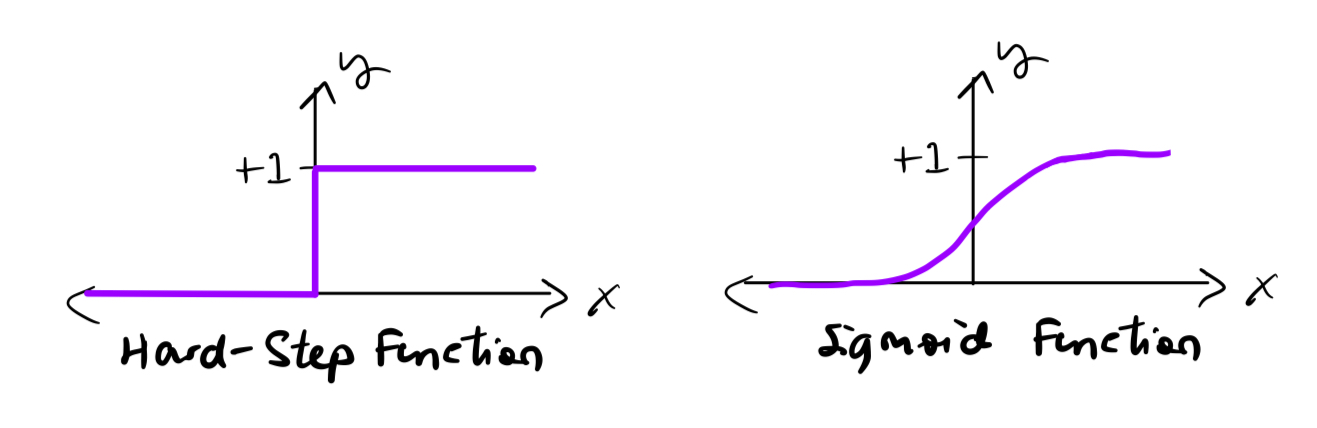 *Comparison of the step function (perceptron) and the sigmoid function (logistic regression).*
### Logistic Regression vs Perceptron
*Comparison of the step function (perceptron) and the sigmoid function (logistic regression).*
### Logistic Regression vs Perceptron
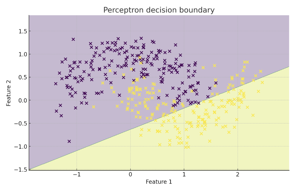
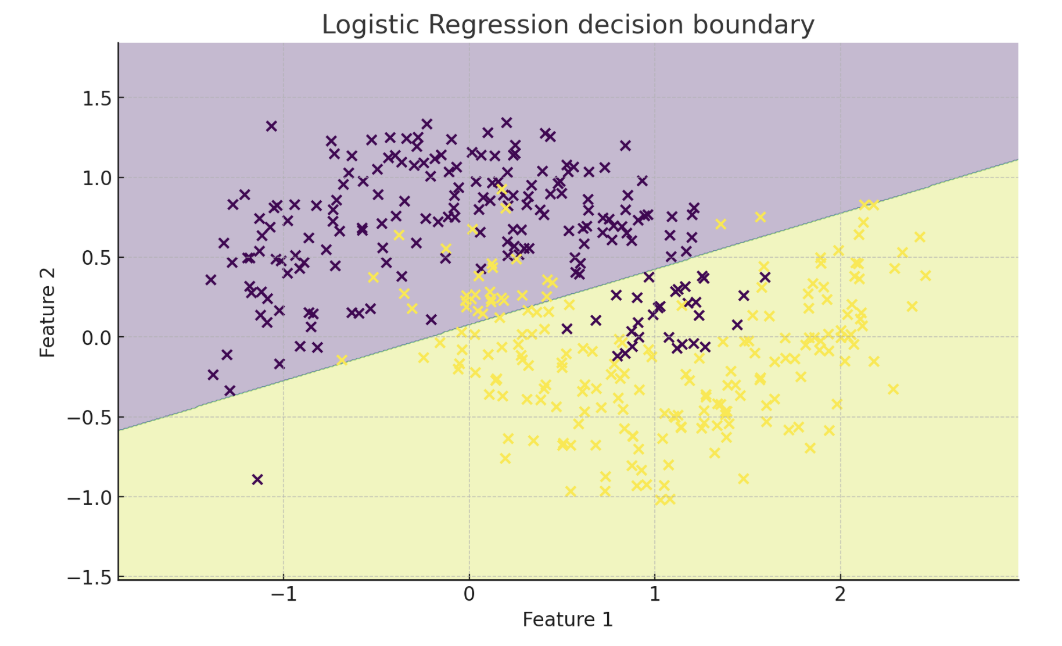 *Perceptron (left) vs logistic regression (right) on non-linearly separable data. Logistic regression does not require the classes to be linearly separable, but its decision boundary is still linear.*
| Model | Output | Updates on | Assumes Linearly Separable? | Training Method |
|---------------------|---------------------|----------------|------------------------------|------------------------|
| **Perceptron** | {-1, +1} | Mistakes only | Yes | Mistake-driven update |
| **Logistic Regression** | [0, 1] (probability) | All examples | No | Gradient descent |
---
## Loss Functions and Maximum Likelihood Estimation
Now that our model outputs probabilities, we need a way to measure how well it performs. This is the purpose of a **loss function**.
### Binary Cross-Entropy (Log Loss)
For binary classification with true label $ y_i \in \{0, 1\} $ and predicted probability $ \hat{y}_i = \sigma(\mathbf{w}^\top \mathbf{x}_i + b) $, the per-example loss is:
$$
\ell(\mathbf{x}_i, y_i) = -\left[ y_i \log(\hat{y}_i) + (1 - y_i) \log(1 - \hat{y}_i) \right]
$$
This loss:
- Is **small** when $ \hat{y}_i $ is close to $ y_i $
- Is **large** when $ \hat{y}_i $ is confidently wrong
- Is **smooth and convex**, allowing gradient descent to work effectively
#### Gradient of the Log Loss
The gradient has a particularly simple form:
$$
\frac{\partial \ell}{\partial \mathbf{w}} = (\hat{y}_i - y_i)\,\mathbf{x}_i, \qquad
\frac{\partial \ell}{\partial b} = \hat{y}_i - y_i
$$
#### Multiclass Extension (Softmax)
For $ K > 2 $ classes, we compute linear scores $ a_k = \mathbf{w}_k^\top \mathbf{x} + b_k $ and transform them with **softmax**:
$$
P(y = k \mid \mathbf{x}) = \frac{e^{a_k}}{\sum_{j=1}^K e^{a_j}}
$$
The per-example loss becomes the **cross-entropy**:
$$
\ell(\mathbf{x}_i, y_i) = -\sum_{k=1}^K \mathbf{1}\{y_i = k\}\,\log P(y = k \mid \mathbf{x}_i)
$$
### Connection to Maximum Likelihood Estimation
Logistic regression models $ P(y = 1 \mid \mathbf{x}) = \sigma(\mathbf{w}^\top \mathbf{x} + b) $. Given a dataset $ D = \{(\mathbf{x}_i, y_i)\}_{i=1}^N $, the likelihood of the data is:
$$
\prod_{i=1}^N \hat{y}_i^{\,y_i} (1 - \hat{y}_i)^{1 - y_i}
$$
To find the best parameters, we **maximize** this likelihood -- or equivalently, **minimize the negative log-likelihood**, which is the total loss over the dataset:
$$
\mathcal{L}(D) = \sum_{(\mathbf{x}_i, y_i) \in D} \ell(\mathbf{x}_i, y_i)
$$
This is known as **maximum likelihood estimation (MLE)**, and it provides a principled statistical basis for minimizing log loss.
---
## Gradient Descent
Now that we have a differentiable loss function, we can minimize it using **gradient descent**.
### Algorithm
1. Initialize weights $ \mathbf{w} $ and bias $ b $ (usually to zero or small random values).
2. For each iteration $ t $:
- Compute the gradient of the loss with respect to $ \mathbf{w} $ and $ b $.
- Update parameters:
$$
\mathbf{w}^{t+1} \leftarrow \mathbf{w}^t - \eta \frac{\partial \mathcal{L}}{\partial \mathbf{w}}, \quad b^{t+1} \leftarrow b^t - \eta \frac{\partial \mathcal{L}}{\partial b}
$$
Here $ \eta $ is the **learning rate**, which controls how large the update steps are.
### Effect of Learning Rate
| Setting | Effect |
|------------------|-----------------------------------------------------------------------------------------------------------------|
| **Small learning rate** | Slow, steady convergence. Noisy gradients get averaged out. Risk of stalling if training time is limited. |
| **Good learning rate** | Fast convergence with a stable loss curve. |
| **Large learning rate** | Rapid jumps that may overshoot the optimum. Sensitive to outliers. Possible divergence or oscillations. |
### Full-batch vs Mini-batch vs Stochastic
| Variant | Gradient computed on | Pros | Cons |
|----------------------|--------------------------|-----------------------------------------|------------------------------|
| **Full-batch** | Entire dataset (N) | Stable, exact gradient | Slow on large N |
| **Mini-batch** | Subset (e.g., 32--512) | Faster; GPU-friendly | Moderate noise |
| **Stochastic (SGD)** | Single example | Cheapest step; escapes shallow minima | Very noisy; needs small learning rate |
Mini-batch SGD is the standard workhorse in deep learning.
### Intuition
- Logistic regression's loss surface is **smooth and convex**, so gradient descent is guaranteed to reach a **global minimum**.
- Unlike the perceptron, which only learns from mistakes, logistic regression learns from **every example**, with larger updates when predictions are more wrong.
---
## Limitations of Linear Models
While linear models are interpretable and fast to train, they have fundamental limitations:
### 1. Only Linearly Separable Data
Linear models can only learn straight-line (or hyperplane) decision boundaries. They cannot capture non-linear patterns.
#### The XOR Problem
| $ x_1 $ | $ x_2 $ | label |
|:----:|:----:|:----:|
| 0 | 0 | 0 |
| 0 | 1 | 1 |
| 1 | 0 | 1 |
| 1 | 1 | 0 |
*Perceptron (left) vs logistic regression (right) on non-linearly separable data. Logistic regression does not require the classes to be linearly separable, but its decision boundary is still linear.*
| Model | Output | Updates on | Assumes Linearly Separable? | Training Method |
|---------------------|---------------------|----------------|------------------------------|------------------------|
| **Perceptron** | {-1, +1} | Mistakes only | Yes | Mistake-driven update |
| **Logistic Regression** | [0, 1] (probability) | All examples | No | Gradient descent |
---
## Loss Functions and Maximum Likelihood Estimation
Now that our model outputs probabilities, we need a way to measure how well it performs. This is the purpose of a **loss function**.
### Binary Cross-Entropy (Log Loss)
For binary classification with true label $ y_i \in \{0, 1\} $ and predicted probability $ \hat{y}_i = \sigma(\mathbf{w}^\top \mathbf{x}_i + b) $, the per-example loss is:
$$
\ell(\mathbf{x}_i, y_i) = -\left[ y_i \log(\hat{y}_i) + (1 - y_i) \log(1 - \hat{y}_i) \right]
$$
This loss:
- Is **small** when $ \hat{y}_i $ is close to $ y_i $
- Is **large** when $ \hat{y}_i $ is confidently wrong
- Is **smooth and convex**, allowing gradient descent to work effectively
#### Gradient of the Log Loss
The gradient has a particularly simple form:
$$
\frac{\partial \ell}{\partial \mathbf{w}} = (\hat{y}_i - y_i)\,\mathbf{x}_i, \qquad
\frac{\partial \ell}{\partial b} = \hat{y}_i - y_i
$$
#### Multiclass Extension (Softmax)
For $ K > 2 $ classes, we compute linear scores $ a_k = \mathbf{w}_k^\top \mathbf{x} + b_k $ and transform them with **softmax**:
$$
P(y = k \mid \mathbf{x}) = \frac{e^{a_k}}{\sum_{j=1}^K e^{a_j}}
$$
The per-example loss becomes the **cross-entropy**:
$$
\ell(\mathbf{x}_i, y_i) = -\sum_{k=1}^K \mathbf{1}\{y_i = k\}\,\log P(y = k \mid \mathbf{x}_i)
$$
### Connection to Maximum Likelihood Estimation
Logistic regression models $ P(y = 1 \mid \mathbf{x}) = \sigma(\mathbf{w}^\top \mathbf{x} + b) $. Given a dataset $ D = \{(\mathbf{x}_i, y_i)\}_{i=1}^N $, the likelihood of the data is:
$$
\prod_{i=1}^N \hat{y}_i^{\,y_i} (1 - \hat{y}_i)^{1 - y_i}
$$
To find the best parameters, we **maximize** this likelihood -- or equivalently, **minimize the negative log-likelihood**, which is the total loss over the dataset:
$$
\mathcal{L}(D) = \sum_{(\mathbf{x}_i, y_i) \in D} \ell(\mathbf{x}_i, y_i)
$$
This is known as **maximum likelihood estimation (MLE)**, and it provides a principled statistical basis for minimizing log loss.
---
## Gradient Descent
Now that we have a differentiable loss function, we can minimize it using **gradient descent**.
### Algorithm
1. Initialize weights $ \mathbf{w} $ and bias $ b $ (usually to zero or small random values).
2. For each iteration $ t $:
- Compute the gradient of the loss with respect to $ \mathbf{w} $ and $ b $.
- Update parameters:
$$
\mathbf{w}^{t+1} \leftarrow \mathbf{w}^t - \eta \frac{\partial \mathcal{L}}{\partial \mathbf{w}}, \quad b^{t+1} \leftarrow b^t - \eta \frac{\partial \mathcal{L}}{\partial b}
$$
Here $ \eta $ is the **learning rate**, which controls how large the update steps are.
### Effect of Learning Rate
| Setting | Effect |
|------------------|-----------------------------------------------------------------------------------------------------------------|
| **Small learning rate** | Slow, steady convergence. Noisy gradients get averaged out. Risk of stalling if training time is limited. |
| **Good learning rate** | Fast convergence with a stable loss curve. |
| **Large learning rate** | Rapid jumps that may overshoot the optimum. Sensitive to outliers. Possible divergence or oscillations. |
### Full-batch vs Mini-batch vs Stochastic
| Variant | Gradient computed on | Pros | Cons |
|----------------------|--------------------------|-----------------------------------------|------------------------------|
| **Full-batch** | Entire dataset (N) | Stable, exact gradient | Slow on large N |
| **Mini-batch** | Subset (e.g., 32--512) | Faster; GPU-friendly | Moderate noise |
| **Stochastic (SGD)** | Single example | Cheapest step; escapes shallow minima | Very noisy; needs small learning rate |
Mini-batch SGD is the standard workhorse in deep learning.
### Intuition
- Logistic regression's loss surface is **smooth and convex**, so gradient descent is guaranteed to reach a **global minimum**.
- Unlike the perceptron, which only learns from mistakes, logistic regression learns from **every example**, with larger updates when predictions are more wrong.
---
## Limitations of Linear Models
While linear models are interpretable and fast to train, they have fundamental limitations:
### 1. Only Linearly Separable Data
Linear models can only learn straight-line (or hyperplane) decision boundaries. They cannot capture non-linear patterns.
#### The XOR Problem
| $ x_1 $ | $ x_2 $ | label |
|:----:|:----:|:----:|
| 0 | 0 | 0 |
| 0 | 1 | 1 |
| 1 | 0 | 1 |
| 1 | 1 | 0 |
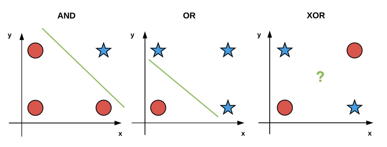 *Both AND and OR contain data that is linearly separable in 2D. However, the XOR problem is not linearly separable -- no single straight line can separate the positive and negative points.*
*[Image credit: Kilian Q. Weinberger and Jennifer J. Sun via [CS 4782](https://www.cs.cornell.edu/courses/cs4782/2025sp/slides/pdf/week1_2_slides.pdf)]*
### 2. Feature Engineering is Essential
Linear models rely on the right input representation. If the raw features do not make the data linearly separable, the model will perform poorly.
### 3. Sensitivity to Outliers
With gradient-based loss functions, outliers can cause large updates. Regularization and robust loss functions can help.
### Overcoming These Limitations
1. **Feature engineering**: Construct new features (e.g., add $ x_1 x_2 $) so the data become separable in a higher-dimensional space.
2. **Kernel methods**: Implicitly project the data into a higher-dimensional space where it becomes linearly separable.
3. **Non-linear models**: Use models such as neural networks that can capture non-linear relationships -- covered in the next lecture.
---
## Key Takeaways
- **Classification** learns a mapping from feature vectors to discrete labels by minimizing a loss defined on labeled examples.
- **Linear decision boundaries**: Both Perceptron and Logistic Regression assume a hyperplane can separate the classes.
- Perceptron makes hard $ \{-1, +1\} $ decisions and updates only on mistakes.
- Logistic Regression outputs soft probabilities and refines weights on every example via smooth log loss.
- **Learning signals**: Perceptron's mistake-driven rule is simple but fails on non-separable data. Logistic Regression + Gradient Descent finds a global optimum thanks to a convex loss surface.
- **Learning rate ($ \eta $)**: Too small leads to slow convergence, too large leads to oscillation or divergence.
- **Limits of linearity**: Straight hyperplanes cannot solve problems like XOR without extra feature engineering or non-linear models (neural nets), covered in the next lecture.
---
## Acknowledgements
Notes originally created by Rachael Chen (rlc355), Tasmin Symons (tks39), Rayhan Khanna, and Emma Li.
## References
1. [Classification Recap, Linear Models Slides](https://www.cs.cornell.edu/courses/cs4782/2025sp/slides/pdf/week1_2_slides.pdf) (CS 4/5782: Deep Learning, Spring 2025)
2. [CS 4780 Lecture Notes on the Perceptron](https://www.cs.cornell.edu/courses/cs4780/2024sp/lectures/lecturenote03.html) (CS 4780, Spring 2024)
*Both AND and OR contain data that is linearly separable in 2D. However, the XOR problem is not linearly separable -- no single straight line can separate the positive and negative points.*
*[Image credit: Kilian Q. Weinberger and Jennifer J. Sun via [CS 4782](https://www.cs.cornell.edu/courses/cs4782/2025sp/slides/pdf/week1_2_slides.pdf)]*
### 2. Feature Engineering is Essential
Linear models rely on the right input representation. If the raw features do not make the data linearly separable, the model will perform poorly.
### 3. Sensitivity to Outliers
With gradient-based loss functions, outliers can cause large updates. Regularization and robust loss functions can help.
### Overcoming These Limitations
1. **Feature engineering**: Construct new features (e.g., add $ x_1 x_2 $) so the data become separable in a higher-dimensional space.
2. **Kernel methods**: Implicitly project the data into a higher-dimensional space where it becomes linearly separable.
3. **Non-linear models**: Use models such as neural networks that can capture non-linear relationships -- covered in the next lecture.
---
## Key Takeaways
- **Classification** learns a mapping from feature vectors to discrete labels by minimizing a loss defined on labeled examples.
- **Linear decision boundaries**: Both Perceptron and Logistic Regression assume a hyperplane can separate the classes.
- Perceptron makes hard $ \{-1, +1\} $ decisions and updates only on mistakes.
- Logistic Regression outputs soft probabilities and refines weights on every example via smooth log loss.
- **Learning signals**: Perceptron's mistake-driven rule is simple but fails on non-separable data. Logistic Regression + Gradient Descent finds a global optimum thanks to a convex loss surface.
- **Learning rate ($ \eta $)**: Too small leads to slow convergence, too large leads to oscillation or divergence.
- **Limits of linearity**: Straight hyperplanes cannot solve problems like XOR without extra feature engineering or non-linear models (neural nets), covered in the next lecture.
---
## Acknowledgements
Notes originally created by Rachael Chen (rlc355), Tasmin Symons (tks39), Rayhan Khanna, and Emma Li.
## References
1. [Classification Recap, Linear Models Slides](https://www.cs.cornell.edu/courses/cs4782/2025sp/slides/pdf/week1_2_slides.pdf) (CS 4/5782: Deep Learning, Spring 2025)
2. [CS 4780 Lecture Notes on the Perceptron](https://www.cs.cornell.edu/courses/cs4780/2024sp/lectures/lecturenote03.html) (CS 4780, Spring 2024)