# MLP, SGD, and Optimization
## Multilayer Perceptron
### Background
Multilayer perceptrons (MLPs) are a type of neural network that serve as the fundamental architecture for many deep learning algorithms. They consist of a series of fully connected layers of nodes, or “neurons.” With a sufficient number of nodes, MLPs can approximate any continuous function and are useful in a number of applications, including: classification, regression, image recognition, and natural language processing (NLP).
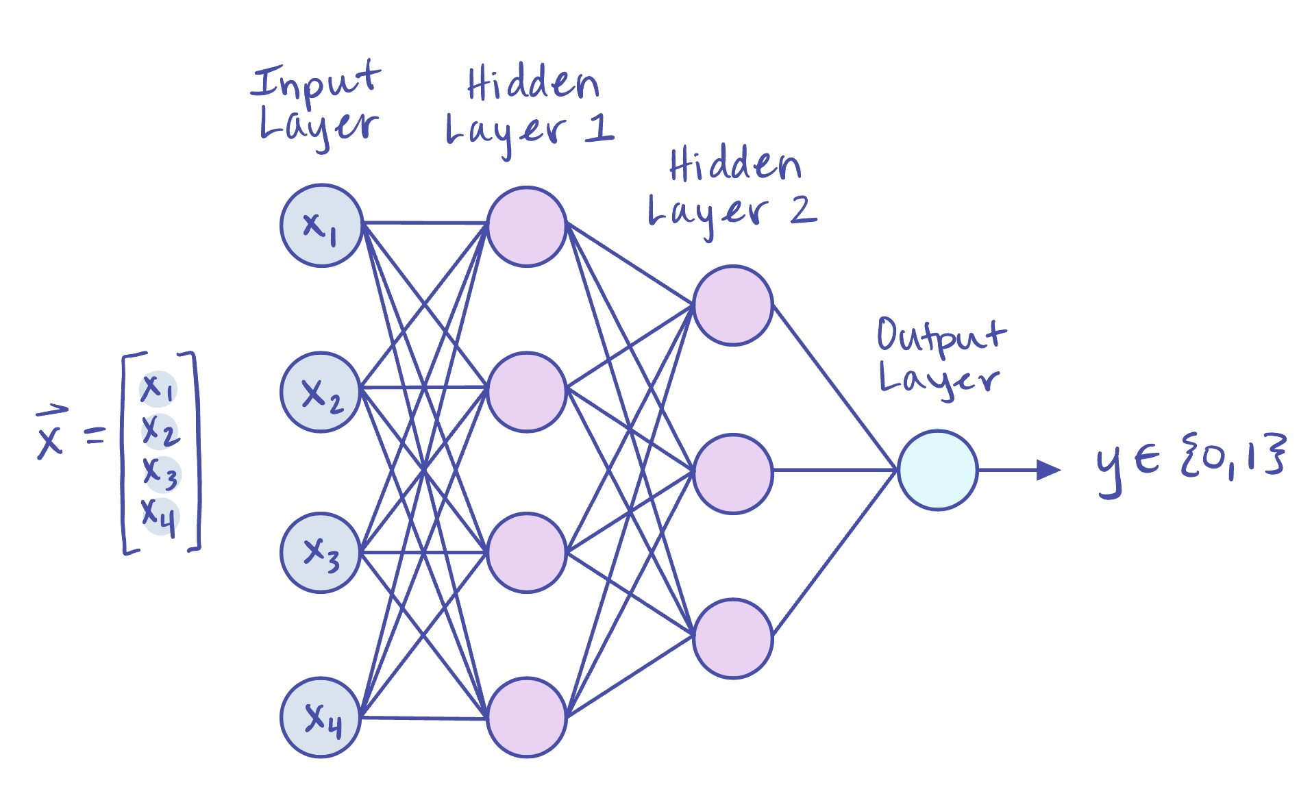 **Figure 1:** A simple MLP with two hidden layers that performs binary classification.
During **training**, the network performs a *forward pass*: an input vector $ \mathbf{x} \in \mathbb{R}^{d} $ is multiplied by a learnable weight matrix, shifted by a bias, and passed through an activation function to produce the input to the next layer. This process repeats layer by layer until the network outputs a final prediction $ \mathbf{\hat{y}} $. Once we have our prediction $ \mathbf{\hat{y}} $, we use our chosen loss function to measure the discrepancy between $ \hat{\mathbf{y}} $ and the target $ \mathbf{y} $. We then perform a *backward pass*, in which backpropagation computes the gradients of the loss function with respect to the network's weights and biases. The chosen optimizer then uses these gradients to update the parameters.
During **testing** (or inference), we just perform a single forward pass with $ \mathbf{x} \in \mathbb{R}^d $ to generate our prediction $ \hat{\mathbf{y}} $.
### A Note on Notation
Below is an explanation of the notation we will adopt for the remainder of the notes. For each layer $ l \in \{1,2,...,L\} $ of an MLP with $ L $ total layers, we have the following:
| Notation | Description |
| :---: | :--- |
| $ \mathbf{z}^{[l-1]} $ | $ \mathbf{z}^{[l-1]} $ is the output from the previous layer $ l-1 $, and thus the input vector to this layer $ l $ (in the very first layer $ l=1 $, we simply set $ \mathbf{z}^{[0]}=\mathbf{x} $, the input vector to the network) |
| $ \mathbf{a}^{[l]} $ | $ \mathbf{a}^{[l]}=\mathbf{W}^{[l]}\mathbf{z}^{[l-1]} + \mathbf{b}^{[l]} $ is the result of multiplying the input $ \mathbf{z}^{[l-1]} $ by the weight matrix $ \mathbf{W}^{[l]} $ for this layer and adding the bias $ \mathbf{b}^{[l]} $ |
| $ \mathbf{z}^{[l]} $ | $ \mathbf{z}^{[l]}=\sigma(\mathbf{a}^{[l]}) $ is the output of this layer $ l $, which we get by applying an activation function $ \sigma(\cdot) $ element-wise to $ \mathbf{a}^{[l]} $ |
### Forward Pass
#### Through a Single Layer
We consider a forward pass through a single layer $ l \in \{1,2,...,L\} $ of an MLP with $ L $ total layers.
1. **Applying Weights and Bias**: We first multiply our input vector $ \mathbf{z}^{[l-1]} $ by the learned weight matrix for this layer $ \mathbf{W}^{[l]} $, and add the bias $ \mathbf{b^{[l]}} $. This gives us $ \mathbf{a}^{[l]}=\mathbf{W}^{[l]}\mathbf{z}^{[l-1]} + \mathbf{b}^{[l]} $ (Note: if we know our input $ \mathbf{z}^{[l-1]} \in \mathbb{R^m} $ and our output $ \mathbf{z}^{[l]} \in \mathbb{R^n} $, then the weight matrix $ \mathbf{W}^{[l]} \in \mathbb{R}^{n \times m} $)
2. **Activation Function**: We now apply an activation function $ \sigma(\cdot) $ element-wise to $ \mathbf{a}^{[l]} $, which gives us our layer's output $ \mathbf{z}^{[l]}=\sigma(\mathbf{a}^{[l]}) $. Then $ \mathbf{z^{[l]}} $ is the input to layer $ l+1 $. See below for examples of activation functions.
If we "zoom in" on a single node, we see that each node first computes a weighted sum of the elements of $ \mathbf{z}^{[l-1]} $. Once we add the bias and apply the activation function, we call the final result the node's activation, which is an element of $ \mathbf{z}^{[l]} $, the output of this layer $ l $ (and the input to the $ l+1 $ layer).
**Figure 1:** A simple MLP with two hidden layers that performs binary classification.
During **training**, the network performs a *forward pass*: an input vector $ \mathbf{x} \in \mathbb{R}^{d} $ is multiplied by a learnable weight matrix, shifted by a bias, and passed through an activation function to produce the input to the next layer. This process repeats layer by layer until the network outputs a final prediction $ \mathbf{\hat{y}} $. Once we have our prediction $ \mathbf{\hat{y}} $, we use our chosen loss function to measure the discrepancy between $ \hat{\mathbf{y}} $ and the target $ \mathbf{y} $. We then perform a *backward pass*, in which backpropagation computes the gradients of the loss function with respect to the network's weights and biases. The chosen optimizer then uses these gradients to update the parameters.
During **testing** (or inference), we just perform a single forward pass with $ \mathbf{x} \in \mathbb{R}^d $ to generate our prediction $ \hat{\mathbf{y}} $.
### A Note on Notation
Below is an explanation of the notation we will adopt for the remainder of the notes. For each layer $ l \in \{1,2,...,L\} $ of an MLP with $ L $ total layers, we have the following:
| Notation | Description |
| :---: | :--- |
| $ \mathbf{z}^{[l-1]} $ | $ \mathbf{z}^{[l-1]} $ is the output from the previous layer $ l-1 $, and thus the input vector to this layer $ l $ (in the very first layer $ l=1 $, we simply set $ \mathbf{z}^{[0]}=\mathbf{x} $, the input vector to the network) |
| $ \mathbf{a}^{[l]} $ | $ \mathbf{a}^{[l]}=\mathbf{W}^{[l]}\mathbf{z}^{[l-1]} + \mathbf{b}^{[l]} $ is the result of multiplying the input $ \mathbf{z}^{[l-1]} $ by the weight matrix $ \mathbf{W}^{[l]} $ for this layer and adding the bias $ \mathbf{b}^{[l]} $ |
| $ \mathbf{z}^{[l]} $ | $ \mathbf{z}^{[l]}=\sigma(\mathbf{a}^{[l]}) $ is the output of this layer $ l $, which we get by applying an activation function $ \sigma(\cdot) $ element-wise to $ \mathbf{a}^{[l]} $ |
### Forward Pass
#### Through a Single Layer
We consider a forward pass through a single layer $ l \in \{1,2,...,L\} $ of an MLP with $ L $ total layers.
1. **Applying Weights and Bias**: We first multiply our input vector $ \mathbf{z}^{[l-1]} $ by the learned weight matrix for this layer $ \mathbf{W}^{[l]} $, and add the bias $ \mathbf{b^{[l]}} $. This gives us $ \mathbf{a}^{[l]}=\mathbf{W}^{[l]}\mathbf{z}^{[l-1]} + \mathbf{b}^{[l]} $ (Note: if we know our input $ \mathbf{z}^{[l-1]} \in \mathbb{R^m} $ and our output $ \mathbf{z}^{[l]} \in \mathbb{R^n} $, then the weight matrix $ \mathbf{W}^{[l]} \in \mathbb{R}^{n \times m} $)
2. **Activation Function**: We now apply an activation function $ \sigma(\cdot) $ element-wise to $ \mathbf{a}^{[l]} $, which gives us our layer's output $ \mathbf{z}^{[l]}=\sigma(\mathbf{a}^{[l]}) $. Then $ \mathbf{z^{[l]}} $ is the input to layer $ l+1 $. See below for examples of activation functions.
If we "zoom in" on a single node, we see that each node first computes a weighted sum of the elements of $ \mathbf{z}^{[l-1]} $. Once we add the bias and apply the activation function, we call the final result the node's activation, which is an element of $ \mathbf{z}^{[l]} $, the output of this layer $ l $ (and the input to the $ l+1 $ layer).
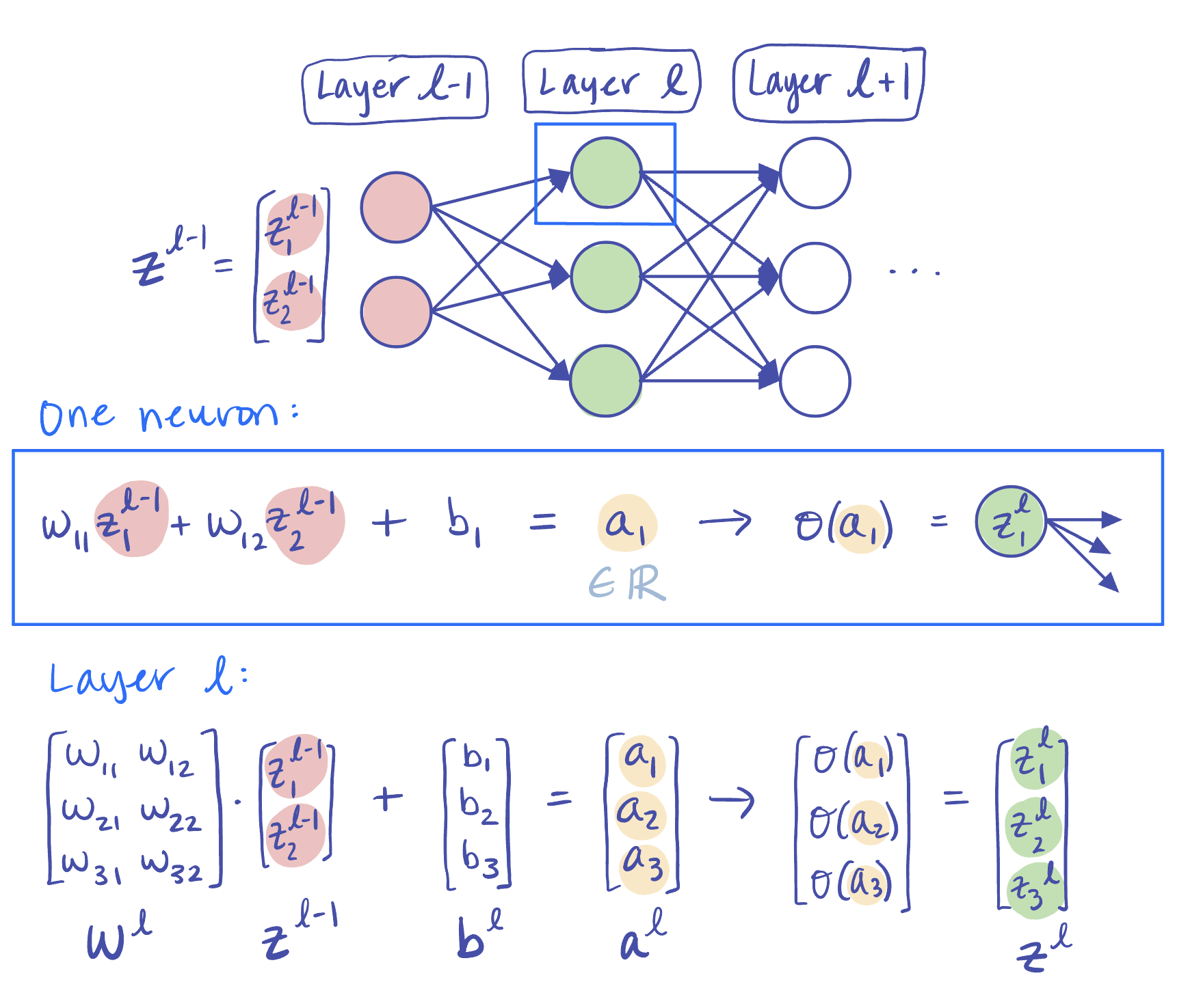 **Figure 2:** Illustration of a forward pass through a single layer $ l $ of an MLP, showing a sample calculation for $ \mathbb{a}^{[l]} $ and $ \mathbb{z}^{[l]} $.
#### Activation Functions
Selecting an appropriate activation function has important ramifications for the behavior of our layer. Setting $ \sigma(\cdot) $ as a step function, for example, turns each node into the classic Perceptron, which can only learn a linear decision boundary. Furthermore, the step function has a zero gradient everywhere (except at $ x=0 $, where it is undefined), making it impractical for learning. Commonly used activation functions, which are both non-linear and differentiable1, are listed below:
| Name | Formulation | Graph | Range | Notes |
| --- | --- | --- | --- | --- |
| **ReLU** (Rectified Linear Unit) | $ \sigma(a) = \max(0,a) $ |
**Figure 2:** Illustration of a forward pass through a single layer $ l $ of an MLP, showing a sample calculation for $ \mathbb{a}^{[l]} $ and $ \mathbb{z}^{[l]} $.
#### Activation Functions
Selecting an appropriate activation function has important ramifications for the behavior of our layer. Setting $ \sigma(\cdot) $ as a step function, for example, turns each node into the classic Perceptron, which can only learn a linear decision boundary. Furthermore, the step function has a zero gradient everywhere (except at $ x=0 $, where it is undefined), making it impractical for learning. Commonly used activation functions, which are both non-linear and differentiable1, are listed below:
| Name | Formulation | Graph | Range | Notes |
| --- | --- | --- | --- | --- |
| **ReLU** (Rectified Linear Unit) | $ \sigma(a) = \max(0,a) $ | 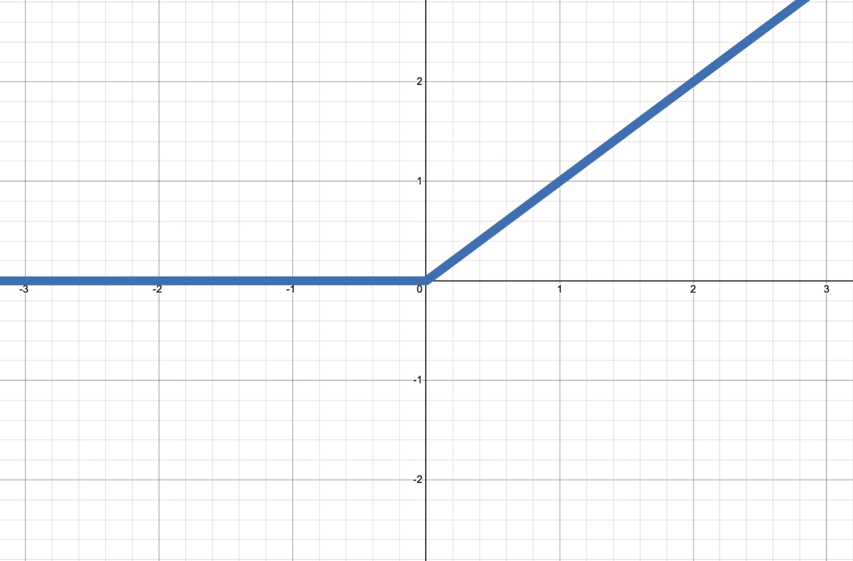 |$ [0,\infty) $ | Most common default activation function in hidden layers of neural networks
| Sigmoid | $ \sigma(a)=\frac{1}{1+e^{-a}} $ |
|$ [0,\infty) $ | Most common default activation function in hidden layers of neural networks
| Sigmoid | $ \sigma(a)=\frac{1}{1+e^{-a}} $ | 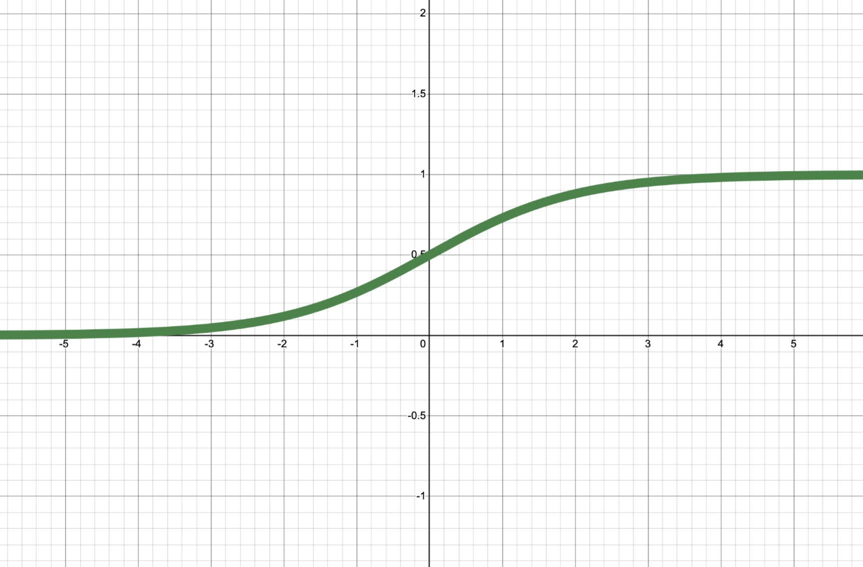 |$ (0,1) $ | Useful for output layer of binary classification problems|
| Tanh (Hyperbolic Tangent) | $ \sigma(a)=\frac{e^a - e^{-a}}{e^a+e^{-a}} $ |
|$ (0,1) $ | Useful for output layer of binary classification problems|
| Tanh (Hyperbolic Tangent) | $ \sigma(a)=\frac{e^a - e^{-a}}{e^a+e^{-a}} $ | 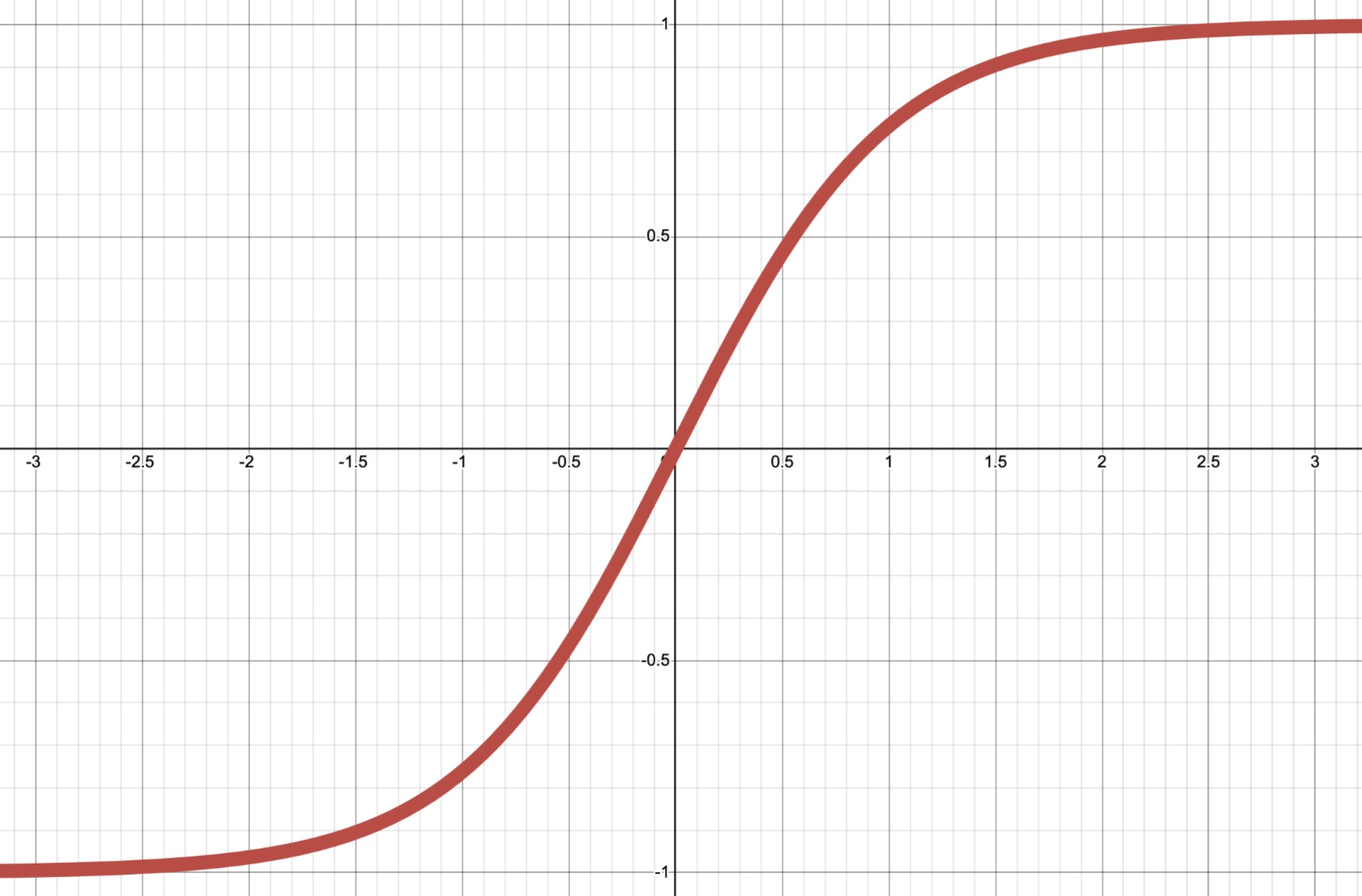 |$ (-1,1) $ | Used in Recurrent Neural Networks (RNNs) and GANs; more computationally expensive than ReLU
1 While ReLU is technically not differentiable at zero, setting the derivative at $ x=0 $ to $ 0 $ works well in practice. Alternatively, there are also variations on ReLU, such as Sigmoid Linear Unit (SiLU) or Gaussian Error Linear Unit (GELU) that are smooth (see the [PyTorch docs](https://docs.pytorch.org/docs/stable/nn.html#non-linear-activations-weighted-sum-nonlinearity) for more information).
### Loss Functions
Once we complete our forward pass, we generate a final prediction $ \mathbf{\hat{y}} $. During training, we need to quantify the difference between our predicted value $ \mathbf{\hat{y}} $ and the ground truth $ \mathbf{y} $ before we adjust the weights of our MLP. That is, we need a loss function.
Consider a training dataset $ \mathcal{D}_{TR}=\{\mathbf{x_i},\mathbf{y_i}\}_{i=0}^n $ where $ \mathbf{y_i} $ and $ \mathbf{\hat{y}_i} $ are the true label and predicted label, respectively, for a point $ \mathbf{x_i} $. Assuming no regularization, our goal is to minimize the loss:
$$ \min_{\mathbf{w}} \mathcal{L}(\mathbf{w};\mathcal{D}_{TR})=\frac{1}{n}\sum_{i}^n \ell(\mathbf{\hat{y}_i},\mathbf{y_i}) $$
where $ \ell(\cdot) $ depends on our choice of loss function. The two most common loss functions for MLPs are:
* __Binary Cross-Entropy (BCE, or Log Loss):__ BCE loss is commonly used in binary classification settings and is formulated as:
$$\mathcal{L}(\mathbf{w};\mathcal{D}_{TR})=-\frac{1}{n}\sum_{i}^n\mathbf{y_i}\log(\mathbf{\hat{y}_i})+(1-\mathbf{y_i})\log(1-\mathbf{\hat{y}_i})$$
* __Mean Squared Error (MSE):__ MSE loss is common in regression settings and is formulated as:
$$\mathcal{L}(\mathbf{w};\mathcal{D}_{TR})=\frac{1}{n}\sum_{i}^n(\mathbf{y_i}-\mathbf{\hat{y}_i})^2$$
In practice, we normally send a minibatch of training points through the network and compute the loss over the minibatch (as opposed to summing over the entire dataset or just a single point). The formulations above provide the general calculation for each case.
### Backpropagation
Backpropagation computes gradients of the loss function with respect to a network's weights and biases efficiently, enabling gradient-based optimization.
#### Motivation for Backpropagation
The loss function is a scalar-valued function of many variables that we want to minimize. If the loss were simply $ \mathcal{L}: \mathbb{R} \rightarrow \mathbb{R} $, we could take its derivative, set it to $ 0 $, and solve for a minimizing value $ w \in \mathbb{R} $. In reality, though, the loss functions of MLPs depend on many parameters and define highly non-convex loss surfaces with local minima and saddle points, as illustrated below:
|$ (-1,1) $ | Used in Recurrent Neural Networks (RNNs) and GANs; more computationally expensive than ReLU
1 While ReLU is technically not differentiable at zero, setting the derivative at $ x=0 $ to $ 0 $ works well in practice. Alternatively, there are also variations on ReLU, such as Sigmoid Linear Unit (SiLU) or Gaussian Error Linear Unit (GELU) that are smooth (see the [PyTorch docs](https://docs.pytorch.org/docs/stable/nn.html#non-linear-activations-weighted-sum-nonlinearity) for more information).
### Loss Functions
Once we complete our forward pass, we generate a final prediction $ \mathbf{\hat{y}} $. During training, we need to quantify the difference between our predicted value $ \mathbf{\hat{y}} $ and the ground truth $ \mathbf{y} $ before we adjust the weights of our MLP. That is, we need a loss function.
Consider a training dataset $ \mathcal{D}_{TR}=\{\mathbf{x_i},\mathbf{y_i}\}_{i=0}^n $ where $ \mathbf{y_i} $ and $ \mathbf{\hat{y}_i} $ are the true label and predicted label, respectively, for a point $ \mathbf{x_i} $. Assuming no regularization, our goal is to minimize the loss:
$$ \min_{\mathbf{w}} \mathcal{L}(\mathbf{w};\mathcal{D}_{TR})=\frac{1}{n}\sum_{i}^n \ell(\mathbf{\hat{y}_i},\mathbf{y_i}) $$
where $ \ell(\cdot) $ depends on our choice of loss function. The two most common loss functions for MLPs are:
* __Binary Cross-Entropy (BCE, or Log Loss):__ BCE loss is commonly used in binary classification settings and is formulated as:
$$\mathcal{L}(\mathbf{w};\mathcal{D}_{TR})=-\frac{1}{n}\sum_{i}^n\mathbf{y_i}\log(\mathbf{\hat{y}_i})+(1-\mathbf{y_i})\log(1-\mathbf{\hat{y}_i})$$
* __Mean Squared Error (MSE):__ MSE loss is common in regression settings and is formulated as:
$$\mathcal{L}(\mathbf{w};\mathcal{D}_{TR})=\frac{1}{n}\sum_{i}^n(\mathbf{y_i}-\mathbf{\hat{y}_i})^2$$
In practice, we normally send a minibatch of training points through the network and compute the loss over the minibatch (as opposed to summing over the entire dataset or just a single point). The formulations above provide the general calculation for each case.
### Backpropagation
Backpropagation computes gradients of the loss function with respect to a network's weights and biases efficiently, enabling gradient-based optimization.
#### Motivation for Backpropagation
The loss function is a scalar-valued function of many variables that we want to minimize. If the loss were simply $ \mathcal{L}: \mathbb{R} \rightarrow \mathbb{R} $, we could take its derivative, set it to $ 0 $, and solve for a minimizing value $ w \in \mathbb{R} $. In reality, though, the loss functions of MLPs depend on many parameters and define highly non-convex loss surfaces with local minima and saddle points, as illustrated below:
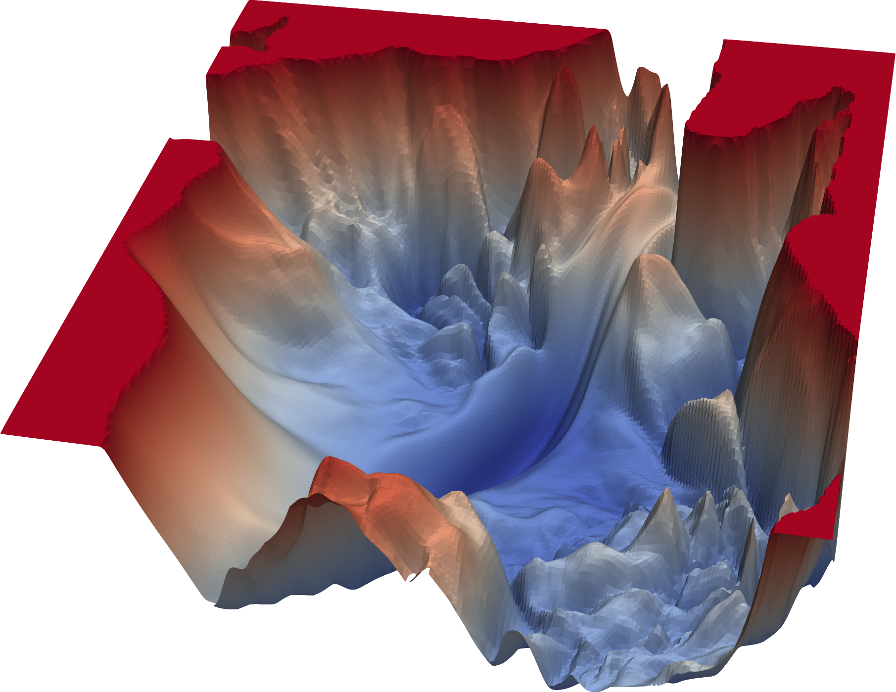 **Figure 4:** Example of a loss surface in a neural network ([University of Maryland, 2018](https://www.cs.umd.edu/~tomg/projects/landscapes/))
The loss is therefore a function of all internal model parameters, $ \mathcal{L}: \mathbb{R}^p \rightarrow \mathbb{R} $. The derivative of such a function is the *gradient*, a vector that points in the direction of steepest *ascent* on the loss surface. To *minimize* the loss, we update parameters (weights and biases) by "stepping" in the opposite direction of the gradient, with the specific update rule determined by the optimizer. Backpropagation is the algorithm that computes these gradients efficiently.
>Computing the gradient efficiently is nontrivial because the loss depends on parameters indirectly through many layers of computation. Backpropagation systematically applies the chain rule to propagate gradients from the loss backwards through the network.
Below is a derivation of backpropagation, with the hope that it gives more insight into the algorithm on the lecture slides:
**Figure 4:** Example of a loss surface in a neural network ([University of Maryland, 2018](https://www.cs.umd.edu/~tomg/projects/landscapes/))
The loss is therefore a function of all internal model parameters, $ \mathcal{L}: \mathbb{R}^p \rightarrow \mathbb{R} $. The derivative of such a function is the *gradient*, a vector that points in the direction of steepest *ascent* on the loss surface. To *minimize* the loss, we update parameters (weights and biases) by "stepping" in the opposite direction of the gradient, with the specific update rule determined by the optimizer. Backpropagation is the algorithm that computes these gradients efficiently.
>Computing the gradient efficiently is nontrivial because the loss depends on parameters indirectly through many layers of computation. Backpropagation systematically applies the chain rule to propagate gradients from the loss backwards through the network.
Below is a derivation of backpropagation, with the hope that it gives more insight into the algorithm on the lecture slides:
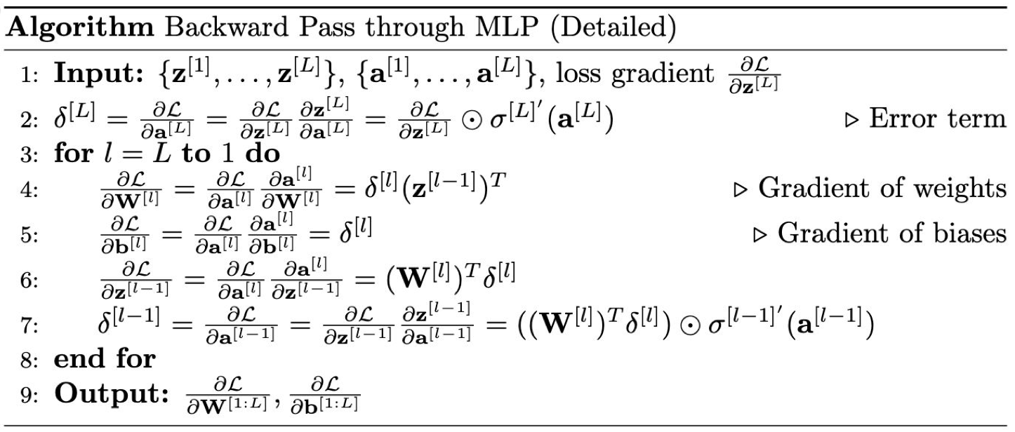 **Figure 3:** Backpropagation algorithm from the "Recap & Multi-Layer Perceptrons" lecture slides ([CS 4782, Cornell University, 2025](https://www.cs.cornell.edu/courses/cs4782/2025sp/slides/pdf/week1_2_slides_complete.pdf))
#### Preliminaries
* **Gradient:** For a scalar-valued function $ f: \mathbb{R}^n \rightarrow \mathbb{R} $, the gradient of $ f $ at a point $ \mathbf{p} \in \mathbb{R}^n $ is the column vector $$ \nabla f(\mathbf{p}) = \begin{bmatrix} \frac{\partial f}{\partial x_1}(\mathbf{p}) \\ \vdots \\ \frac{\partial f}{\partial x_n}(\mathbf{p}) \end{bmatrix} $$ Each component of the gradient is a partial derivative of $ f $ with respect to one coordinate, and together they indicate the direction of steepest increase along $ f $ near $ \mathbf{p} $.
* **Jacobian:** For a vector-valued function $ g: \mathbb{R}^m \rightarrow \mathbb{R}^n $, the Jacobian of $ g $ at a point $ \mathbf{p} \in \mathbb{R}^m $ is $$ \mathbf{J}_g(\mathbf{p}) = \begin{bmatrix} \frac{\partial g_1}{\partial x_1}(\mathbf{p}) & \ldots & \frac{\partial g_1}{\partial x_m}(\mathbf{p}) \\ \vdots & \ddots & \vdots \\ \frac{\partial g_n}{\partial x_1}(\mathbf{p}) & \ldots & \frac{\partial g_n}{\partial x_m}(\mathbf{p}) \end{bmatrix} $$ Each row contains the partial derivatives of one output component $ g_i \in \{g_1, ..., g_n\} $ with respect to all inputs.
* **The Chain Rule:** Let $ f: \mathbb{R}^n \rightarrow \mathbb{R} $ and $ g: \mathbb{R}^m \rightarrow \mathbb{R}^n $ with $ \mathbf{y} = g(\mathbf{x}) $. Then the gradient of $ z=f(g(\mathbf{x})) $ with respect to $ \mathbf{x} $ is given by $$\tag{1} \frac{\partial z}{\partial \mathbf{x}}=\left(\frac{\partial \mathbf{y}}{\partial \mathbf{x}}\right)^T \frac{\partial z}{\partial \mathbf{y}} $$ where $ \frac{\partial \mathbf{y}}{\partial \mathbf{x}} \in \mathbb{R}^{n \times m} $ is the Jacobian of $ g $ and $ \frac{\partial z}{\partial \mathbf{y}} \in \mathbb{R}^n $ is the gradient of $ z $ with respect to $ \mathbf{y} $.
>**Remark 1:** More generally, the chain rule is often written schematically as $$ \tag{2} \frac{\partial \mathbf{z}}{\partial \mathbf{x}} = \frac{\partial \mathbf{z}}{\partial \mathbf{y}} \frac{\partial \mathbf{y}}{\partial \mathbf{x}} $$ where the objects represented by these partial derivatives may be scalars, vectors, or matrices depending on the dimensions of $ \mathbf{z} $, $ \mathbf{y} $, and $ \mathbf{x} $. We will frequently use the formula from Equation (1), where $ z \in \mathbb{R} $ is a scalar and $ \mathbf{x} \in \mathbb{R}^m $, $ \mathbf{y} \in \mathbb{R}^n $ are vectors.
>**Remark 2:** How did we arrive at Equation (1)? This formulation of the chain rule comes from the "Deep Feedforward Networks" chapter (p. 203) of the [Deep Learning Book](https://www.deeplearningbook.org) (Goodfellow et al., 2016), which provides a derivation.
In the context of neural networks, $ g: \mathbb{R}^m \to \mathbb{R}^n $ represents operations performed in layer $ l $ (including weights, biases, and activation functions), and $ f: \mathbb{R}^n \to \mathbb{R} $ is the scalar-valued loss function $ \mathcal{L} $. Backpropagation computes $ \frac{\partial z}{\partial \mathbf{x}} $, the gradient of the loss function with respect to the model's parameters, by repeatedly applying the chain rule.
* **Note on Dimensions:** In the following derivation, we assume $ \mathbf{z}^{[L-1]} \in \mathbb{R}^m $ and $ \mathbf{z}^{[L]} \in \mathbb{R}^n $, meaning that $ \mathbf{W}^{[L]} \in \mathbb{R}^{n \times m} $. We treat gradients as column vectors, as is convention. (And $ \mathbf{v} \in \mathbb{R}^n $ denotes that $ \mathbf{v} $ is an $ n $-dimensional column vector.)
**Setting:** Recall that for layer $ l \in \{1, 2, ..., L \} $, we have $ \mathbf{a}^{[l]} = \mathbf{W}^{[l]}\mathbf{z}^{[l-1]}+\mathbf{b}^{[l]} $ and $ \mathbf{z}^{[l]} = \sigma(\mathbf{a}^{[l]}) $, where $ \sigma: \mathbb{R} \to \mathbb{R} $ is applied element-wise to $ \mathbf{a}^{[l]} $. For the last layer $ L $ of our MLP, that gives us
**Figure 3:** Backpropagation algorithm from the "Recap & Multi-Layer Perceptrons" lecture slides ([CS 4782, Cornell University, 2025](https://www.cs.cornell.edu/courses/cs4782/2025sp/slides/pdf/week1_2_slides_complete.pdf))
#### Preliminaries
* **Gradient:** For a scalar-valued function $ f: \mathbb{R}^n \rightarrow \mathbb{R} $, the gradient of $ f $ at a point $ \mathbf{p} \in \mathbb{R}^n $ is the column vector $$ \nabla f(\mathbf{p}) = \begin{bmatrix} \frac{\partial f}{\partial x_1}(\mathbf{p}) \\ \vdots \\ \frac{\partial f}{\partial x_n}(\mathbf{p}) \end{bmatrix} $$ Each component of the gradient is a partial derivative of $ f $ with respect to one coordinate, and together they indicate the direction of steepest increase along $ f $ near $ \mathbf{p} $.
* **Jacobian:** For a vector-valued function $ g: \mathbb{R}^m \rightarrow \mathbb{R}^n $, the Jacobian of $ g $ at a point $ \mathbf{p} \in \mathbb{R}^m $ is $$ \mathbf{J}_g(\mathbf{p}) = \begin{bmatrix} \frac{\partial g_1}{\partial x_1}(\mathbf{p}) & \ldots & \frac{\partial g_1}{\partial x_m}(\mathbf{p}) \\ \vdots & \ddots & \vdots \\ \frac{\partial g_n}{\partial x_1}(\mathbf{p}) & \ldots & \frac{\partial g_n}{\partial x_m}(\mathbf{p}) \end{bmatrix} $$ Each row contains the partial derivatives of one output component $ g_i \in \{g_1, ..., g_n\} $ with respect to all inputs.
* **The Chain Rule:** Let $ f: \mathbb{R}^n \rightarrow \mathbb{R} $ and $ g: \mathbb{R}^m \rightarrow \mathbb{R}^n $ with $ \mathbf{y} = g(\mathbf{x}) $. Then the gradient of $ z=f(g(\mathbf{x})) $ with respect to $ \mathbf{x} $ is given by $$\tag{1} \frac{\partial z}{\partial \mathbf{x}}=\left(\frac{\partial \mathbf{y}}{\partial \mathbf{x}}\right)^T \frac{\partial z}{\partial \mathbf{y}} $$ where $ \frac{\partial \mathbf{y}}{\partial \mathbf{x}} \in \mathbb{R}^{n \times m} $ is the Jacobian of $ g $ and $ \frac{\partial z}{\partial \mathbf{y}} \in \mathbb{R}^n $ is the gradient of $ z $ with respect to $ \mathbf{y} $.
>**Remark 1:** More generally, the chain rule is often written schematically as $$ \tag{2} \frac{\partial \mathbf{z}}{\partial \mathbf{x}} = \frac{\partial \mathbf{z}}{\partial \mathbf{y}} \frac{\partial \mathbf{y}}{\partial \mathbf{x}} $$ where the objects represented by these partial derivatives may be scalars, vectors, or matrices depending on the dimensions of $ \mathbf{z} $, $ \mathbf{y} $, and $ \mathbf{x} $. We will frequently use the formula from Equation (1), where $ z \in \mathbb{R} $ is a scalar and $ \mathbf{x} \in \mathbb{R}^m $, $ \mathbf{y} \in \mathbb{R}^n $ are vectors.
>**Remark 2:** How did we arrive at Equation (1)? This formulation of the chain rule comes from the "Deep Feedforward Networks" chapter (p. 203) of the [Deep Learning Book](https://www.deeplearningbook.org) (Goodfellow et al., 2016), which provides a derivation.
In the context of neural networks, $ g: \mathbb{R}^m \to \mathbb{R}^n $ represents operations performed in layer $ l $ (including weights, biases, and activation functions), and $ f: \mathbb{R}^n \to \mathbb{R} $ is the scalar-valued loss function $ \mathcal{L} $. Backpropagation computes $ \frac{\partial z}{\partial \mathbf{x}} $, the gradient of the loss function with respect to the model's parameters, by repeatedly applying the chain rule.
* **Note on Dimensions:** In the following derivation, we assume $ \mathbf{z}^{[L-1]} \in \mathbb{R}^m $ and $ \mathbf{z}^{[L]} \in \mathbb{R}^n $, meaning that $ \mathbf{W}^{[L]} \in \mathbb{R}^{n \times m} $. We treat gradients as column vectors, as is convention. (And $ \mathbf{v} \in \mathbb{R}^n $ denotes that $ \mathbf{v} $ is an $ n $-dimensional column vector.)
**Setting:** Recall that for layer $ l \in \{1, 2, ..., L \} $, we have $ \mathbf{a}^{[l]} = \mathbf{W}^{[l]}\mathbf{z}^{[l-1]}+\mathbf{b}^{[l]} $ and $ \mathbf{z}^{[l]} = \sigma(\mathbf{a}^{[l]}) $, where $ \sigma: \mathbb{R} \to \mathbb{R} $ is applied element-wise to $ \mathbf{a}^{[l]} $. For the last layer $ L $ of our MLP, that gives us
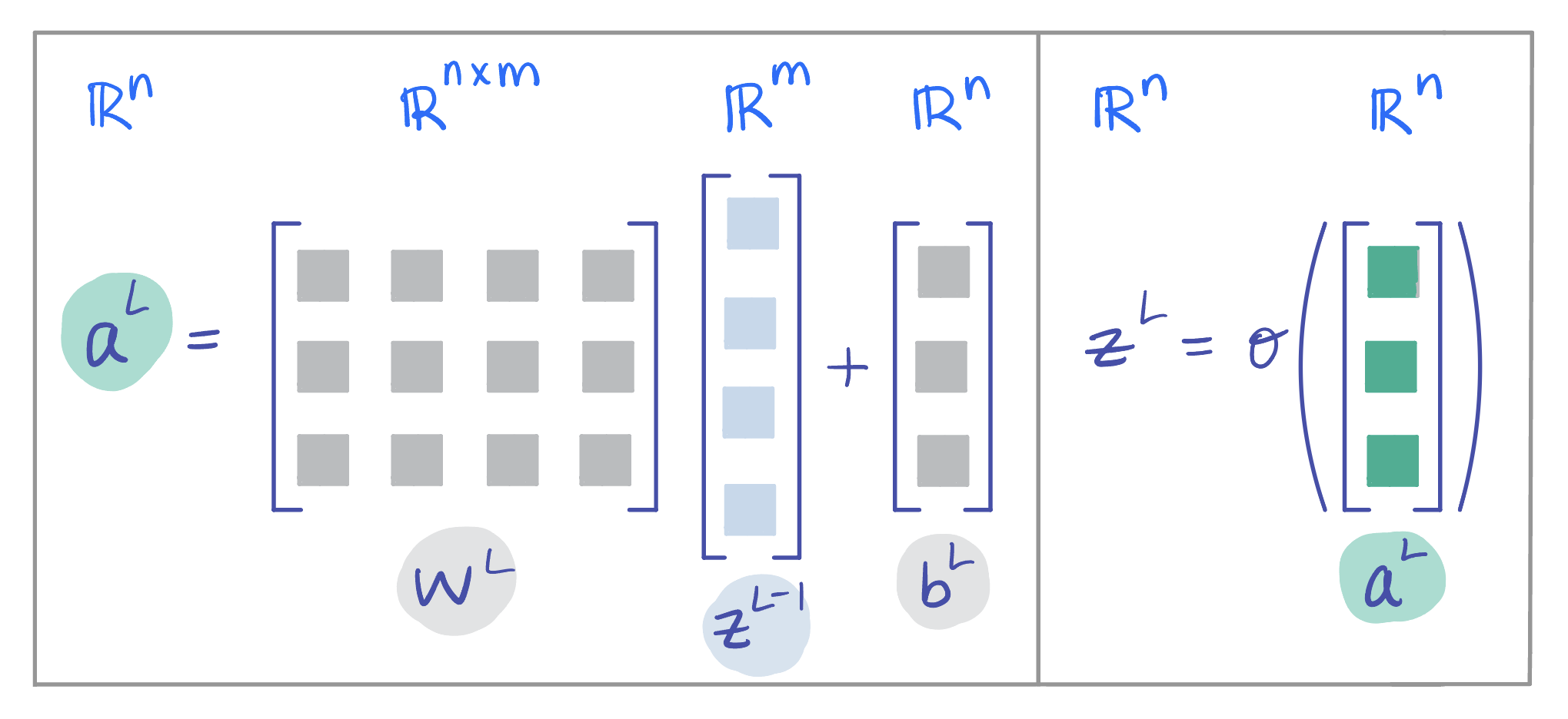 **Figure 4:** Visualization of an example last layer $ L $ of an MLP, with dimensions matching those used in the backpropagation derivation below.
#### Starting at Layer $ L $
With backpropagation, we start at the end of the MLP and work our way *backwards* until we have computed the gradient of $ \mathcal{L}(\cdot) $ with respect to all parameters. Concretely, we want
$$ \frac{\partial \mathcal{L}}{\partial \mathbf{W}^{[l]}} \text{ and } \frac{\partial \mathcal{L}}{\partial \mathbf{b}^{[l]}} \text{ for } l \in \{1, 2, ..., L\}$$
From our forward pass, we currently have $ \mathbf{z}^{[L]} $ (the output of the last layer $ L $), which is equivalent to our prediction $ \mathbf{\hat{y}} $. Thus, we can directly compute $ \frac{\partial \mathcal{L}}{\partial \mathbf{z}^{[L]}} $.
Recall that we have the following structure in our MLP: $ \mathbf{z}^{[L]} $ is a function of $ \mathbf{a}^{[L]} $, which in turn is a function of $ \mathbf{W}^{[L]} $, $ \mathbf{z}^{[L-1]} $, and $ \mathbf{b}^{[L]} $:
**Figure 4:** Visualization of an example last layer $ L $ of an MLP, with dimensions matching those used in the backpropagation derivation below.
#### Starting at Layer $ L $
With backpropagation, we start at the end of the MLP and work our way *backwards* until we have computed the gradient of $ \mathcal{L}(\cdot) $ with respect to all parameters. Concretely, we want
$$ \frac{\partial \mathcal{L}}{\partial \mathbf{W}^{[l]}} \text{ and } \frac{\partial \mathcal{L}}{\partial \mathbf{b}^{[l]}} \text{ for } l \in \{1, 2, ..., L\}$$
From our forward pass, we currently have $ \mathbf{z}^{[L]} $ (the output of the last layer $ L $), which is equivalent to our prediction $ \mathbf{\hat{y}} $. Thus, we can directly compute $ \frac{\partial \mathcal{L}}{\partial \mathbf{z}^{[L]}} $.
Recall that we have the following structure in our MLP: $ \mathbf{z}^{[L]} $ is a function of $ \mathbf{a}^{[L]} $, which in turn is a function of $ \mathbf{W}^{[L]} $, $ \mathbf{z}^{[L-1]} $, and $ \mathbf{b}^{[L]} $:
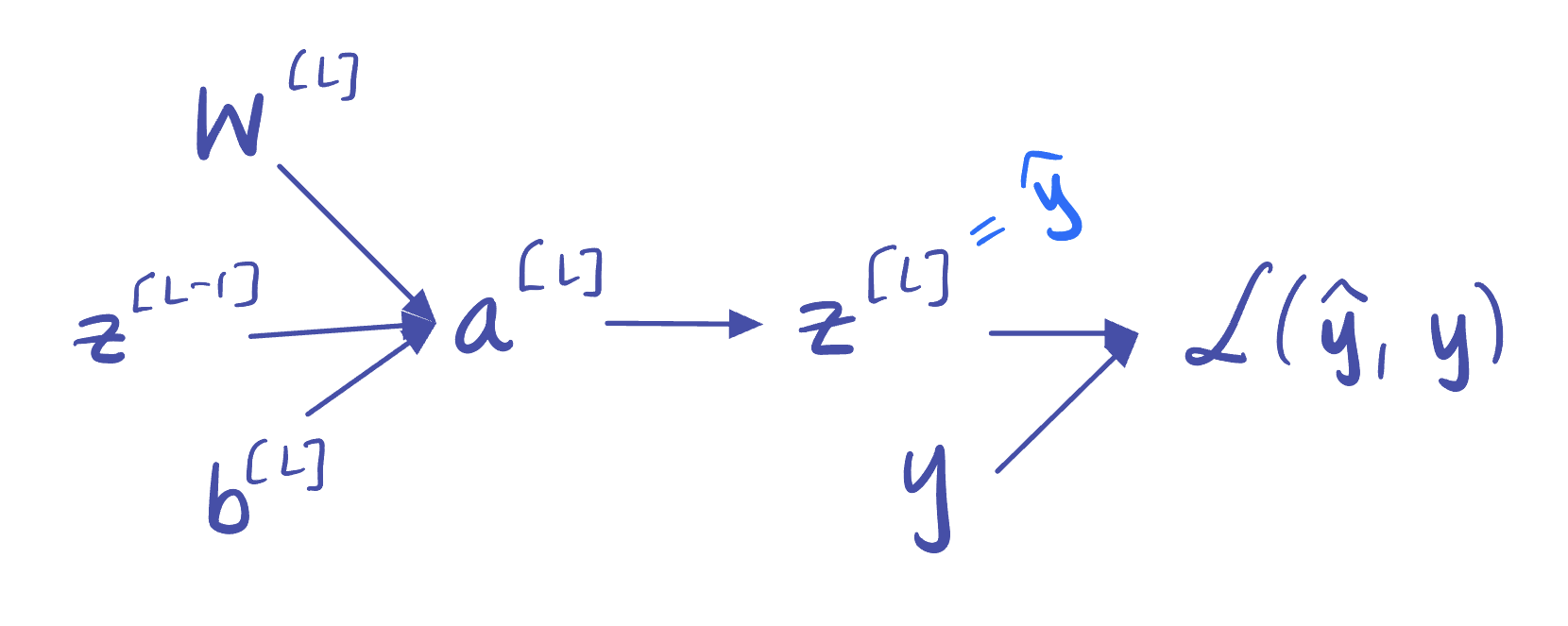 **Figure 5:** Dependency graph for the final layer $ L $ of our MLP.
Hence, the general form of the chain rule tells us that
$$ \frac{\partial \mathcal{L}}{\partial \mathbf{W}^{[L]}}=\frac{\partial \mathcal{L}}{\partial \mathbf{z}^{[L]}} \frac{\partial \mathbf{z}^{[L]}}{\partial \mathbf{a}^{[L]}} \frac{\partial \mathbf{a}^{[L]}}{\partial \mathbf{W}^{[L]}} \ \text{ and } \ \frac{\partial \mathcal{L}}{\partial \mathbf{b}^{[L]}}=\frac{\partial \mathcal{L}}{\partial \mathbf{z}^{[L]}} \frac{\partial \mathbf{z}^{[L]}}{\partial \mathbf{a}^{[L]}} \frac{\partial \mathbf{a}^{[L]}}{\partial \mathbf{b}^{[L]}} $$
We see that $$ \frac{\partial \mathcal{L}}{\partial \mathbf{a}^{[L]}} = \frac{\partial \mathcal{L}}{\partial \mathbf{z}^{[L]}} \frac{\partial \mathbf{z}^{[L]}}{\partial \mathbf{a}^{[L]}} $$
appears in our expressions for $ \frac{\partial \mathcal{L}}{\partial \mathbf{W}^{[L]}} $ and $ \frac{\partial \mathcal{L}}{\partial \mathbf{b}^{[L]}} $, so we compute $ \frac{\partial \mathcal{L}}{\partial \mathbf{a}^{[L]}} = \delta^{[L]} $ first.
#### Line 2: Computing $ \delta^{[L]} $
Using the chain rule from Equation (1), we have
$$ \delta^{[L]}= \frac{\partial \mathcal{L}}{\partial \mathbf{a}^{[L]}} = \left(\frac{\partial \mathbf{z}^{[L]}}{\partial \mathbf{a}^{[L]}} \right)^T \frac{\partial \mathcal{L}}{\partial \mathbf{z}^{[L]}}$$
where $ \delta^{[L]} $ is shorthand for $ \frac{\partial \mathcal{L}}{\partial \mathbf{a}^{[L]}} $.
>**Remark:** Although the final output of the network is typically a scalar, we treat $ \mathbf{z}^{[L]} $ as a (1-dimensional) vector so that the same derivation applies to all layers $ l \in \{1, 2, ..., L-1\} $, where $ \mathbf{z}^{[l]} $ is vector-valued.
We can compute $ \frac{\partial \mathcal{L}}{\partial \mathbf{z}^{[L]}} $ directly. What remains is to compute $ \frac{\partial \mathbf{z}^{[L]}}{\partial \mathbf{a}^{[L]}} $.
Since $ \mathbf{z}^{[L]} = \sigma(\mathbf{a}^{[L]}) $ and $ \mathbf{z}^{[L]}, \mathbf{a}^{[L]} \in \mathbb{R}^n $, the Jacobian is
$$ \frac{\partial \mathbf{z}^{[L]}}{\partial \mathbf{a}^{[L]}} = \begin{bmatrix} \frac{\partial}{\partial a_1^{[L]}} \left[\sigma(a_1^{[L]}) \right] & \ldots & \frac{\partial}{\partial a_n^{[L]}} \left[ \sigma(a_1^{[L]})\right] \\ \vdots & \ddots & \vdots \\ \frac{\partial}{\partial a_1^{[L]}} \left[\sigma(a_n^{[L]})\right] & \ldots & \frac{\partial}{\partial a_n^{[L]}} \left[ \sigma(a_n^{[L]}) \right]\end{bmatrix} = \begin{bmatrix} \sigma'(a_1^{[L]}) & \ldots & 0 \\ \vdots & \ddots & \vdots \\ 0 & \ldots & \sigma'(a_n^{[L]})\end{bmatrix}$$
(a diagonal matrix), which gives us
$$ \left(\frac{\partial \mathbf{z}^{[L]}}{\partial \mathbf{a}^{[L]}} \right)^T \frac{\partial \mathcal{L}}{\partial \mathbf{z}^{[L]}} = \begin{bmatrix} \sigma'(a_1^{[L]}) & \ldots & 0 \\ \vdots & \ddots & \vdots \\ 0 & \ldots & \sigma'(a_n^{[L]})\end{bmatrix} \begin{bmatrix} \frac{\partial \mathcal{L}}{\partial z_1^{[L]}} \\ \vdots \\ \frac{\partial \mathcal{L}}{\partial z_n^{[L]}} \end{bmatrix} = \begin{bmatrix} \frac{\partial \mathcal{L}}{\partial z_1^{[L]}} \cdot \sigma'(a_1^{[L]}) \\ \vdots \\ \frac{\partial \mathcal{L}}{\partial z_n^{[L]}} \cdot \sigma'(a_n^{[L]}) \end{bmatrix} $$
We can rewrite the above using $ \odot $, the symbol for element-wise multiplication, to conclude
$$ \frac{\partial \mathcal{L}}{\partial \mathbf{a}^{[L]}} = \frac{\partial \mathcal{L}}{\partial \mathbf{z}^{[L]}} \odot \sigma'(\mathbf{a}^{[L]}) $$
as expected.
#### Line 4: Computing $ \frac{\partial \mathcal{L}}{\partial \mathbf{W}^{[L]}} $
We have that
$$ \frac{\partial \mathcal{L}}{\partial \mathbf{W}^{[L]}} = \frac{\partial \mathcal{L}}{\partial \mathbf{a}^{[L]}} \frac{\partial \mathbf{a}^{[L]}}{\partial \mathbf{W}^{[L]}} $$
We will not use Equation (1) directly, since we are differentiating with respect to a matrix $ \mathbf{W}^{[L]} \in \mathbb{R}^{n \times m} $ rather than a vector.
>If we flattened $ \mathbf{W}^{[L]} \in \mathbb{R}^{n \times m} $ to an $ nm $-dimensional column vector and used Equation (1), we would get $ \frac{\partial \mathcal{L}}{\partial \mathbf{W}^{[L]}} = \left(\frac{\partial \mathbf{a}^{[L]}}{\partial \mathbf{W}^{[L]}} \right)^T \frac{\partial \mathcal{L}}{\partial \mathbf{a}^{[L]}} $ where the Jacobian $ \frac{\partial \mathbf{a}^{[L]}}{\partial \mathbf{W}^{[L]}} \in \mathbb{R}^{n \times nm} $. This implies $ \frac{\partial \mathcal{L}}{\partial \mathbf{W}^{[L]}} \in \mathbb{R}^{nm} $ would be an $ nm $-dimensonal column vector, which does not match the shape of $ \mathbf{W}^{[L]} \in \mathbb{R}^{n \times m} $ (and, at least in theory, we want these shapes to align).
We would like $ \frac{\partial \mathcal{L}}{\partial \mathbf{W}^{[L]}} $ to also be an $ n \times m $ matrix of the form
$$\frac{\partial \mathcal{L}}{\partial \mathbf{W}^{[L]}} = \begin{bmatrix} \frac{\partial \mathcal{L}}{\partial W_{11}^{[L]}} & \ldots & \frac{\partial \mathcal{L}}{\partial W_{1m}^{[L]}} \\ \vdots & \ddots & \vdots \\ \frac{\partial \mathcal{L}}{\partial W_{n1}^{[L]}} & \ldots & \frac{\partial \mathcal{L}}{\partial W_{nm}^{[L]}} \end{bmatrix}$$
Consider the $ (i,j) $ entry of $ \frac{\partial \mathcal{L}}{\partial \mathbf{W}^{[L]}} $. By the general form of the chain rule,
$$ \frac{\partial \mathcal{L}}{\partial W_{ij}^{[L]}} = \frac{\partial \mathcal{L}}{\partial a_i^{[L]}} \frac{\partial a_i^{[L]}}{\partial W_{ij}^{[L]}} $$
(which we can do because $ a_i $ is the only component of $ \mathbf{a}^{[L]} $ that uses $ W_{ij}^{[L]} $ in its computation). Note that $ \frac{\partial \mathcal{L}}{\partial a_i^{[L]}} $ is the $ i $-th entry of $ \delta^{[L]} $ by definition. Furthermore, observe that
$$ \frac{\partial a_i^{[L]}}{\partial W_{ij}^{[L]}} = \frac{\partial}{\partial W_{ij}^{[L]}} \left[\left(\sum_{k=1}^m W_{ik}^{[L]} z_k^{[L-1]}\right) + b_i^{[L]} \right] = z_j^{[L-1]} $$
Thus, the $ (i,j) $ entry of $ \frac{\partial \mathcal{L}}{\partial \mathbf{W}^{[L]}} $ is given by
$$ \frac{\partial \mathcal{L}}{\partial W_{ij}^{[L]}} = \delta_i^{[L]} z_j^{[L-1]} $$
meaning $ \frac{\partial \mathcal{L}}{\partial \mathbf{W}^{[L]}} $ is equal to the outer product
$$ \frac{\partial \mathcal{L}}{\partial \mathbf{W}^{[L]}} = \delta^{[L]} \left(\mathbf{z}^{[L-1]}\right)^T $$
as expected. (We can confirm that multiplying $ \delta^{[L]} \in \mathbb{R}^{n \times 1} $ and $ (\mathbf{z}^{[L-1]})^T \in \mathbb{R}^{1\times m} $ does indeed yield an $ n \times m $ matrix.)
>**Remark:** This section was from [Computing Neural Network Gradients](https://web.stanford.edu/class/archive/cs/cs224n/cs224n.1184/readings/gradient-notes.pdf) (Kevin Clark, Stanford), which offers another explanation of how to derive $ \frac{\partial \mathcal{L}}{\partial \mathbf{W}^{[L]}} $ on p.3.
#### Line 5: Computing $ \frac{\partial \mathcal{L}}{\partial \mathbf{b}^{[L]}} $
Using the chain rule from Equation (1), we have
$$ \frac{\partial \mathcal{L}}{\partial \mathbf{b}^{[L]}} = \left( \frac{\partial \mathbf{a}^{[L]}}{\partial \mathbf{b}^{[L]}} \right)^T \frac{\partial \mathcal{L}}{\partial \mathbf{a}^{[L]}} $$
We already computed $ \frac{\partial \mathcal{L}}{\partial \mathbf{a}^{[L]}}=\delta^{[L]} $, so we need $ \frac{\partial \mathbf{a}^{[L]}}{\partial \mathbf{b}^{[L]}} $. Since $ \mathbf{a}^{[L]}, \mathbf{b}^{[L]} \in \mathbb{R}^n $, the Jacobian is
$$ \frac{\partial \mathbf{a}^{[L]}}{\partial \mathbf{b}^{[L]}} = \begin{bmatrix} \frac{\partial a_1^{[L]}}{\partial b_1^{[L]}} & \ldots & \frac{\partial a_1^{[L]}}{\partial b_n^{[L]}} \\ \vdots & \ddots & \vdots \\ \frac{\partial a_n^{[L]}}{\partial b_1^{[L]}} & \ldots & \frac{\partial a_n^{[L]}}{\partial b_n^{[L]}} \end{bmatrix} $$
Consider the $ (1,1) $ entry:
$$ \frac{\partial a_1^{[L]}}{\partial b_1^{[L]}} = \frac{\partial}{\partial b_1^{[L]}} \left[ \left(\sum_{j=1}^m W_{1j}^{[L]}z_j^{[L-1]} \right)+ b_1^{[L]}\right] = 1 $$
More generally,
$$\frac{\partial a_i^{[L]}}{\partial b_j^{[L]}}=\begin{cases} 1 & \text{if } i=j \\ 0 & \text{otherwise} \end{cases} \ \Rightarrow \ \frac{\partial \mathbf{a}^{[L]}}{\partial \mathbf{b}^{[L]}} = I_{n \times n}\ $$
so we conclude that
$$ \frac{\partial \mathcal{L}}{\partial \mathbf{b}^{[L]}} = \delta^{[L]} $$
as expected.
#### Line 6: Computing $ \frac{\partial \mathcal{L}}{\partial \mathbf{z}^{[L-1]}} $
>**Why are we computing $ \frac{\partial \mathcal{L}}{\partial \mathbf{z}^{[L-1]}} $?**
If we look ahead to Line 7 in the backpropagation algorithm, we need $ \frac{\partial \mathcal{L}}{\partial \mathbf{z}^{[L-1]}} $ in order to compute $ \delta^{[L-1]} $, which will be key for computing the gradients of the loss with respect to the weights and biases of layer $ L-1 $.
Using the chain rule from Equation (1),
$$ \frac{\partial \mathcal{L}}{\partial \mathbf{z}^{[L-1]}} = \left(\frac{\partial \mathbf{a}^{[L]}}{\partial \mathbf{z}^{[L-1]}} \right)^T \frac{\partial \mathcal{L}}{\partial \mathbf{a}^{[L]}} $$
We already computed $ \frac{\partial \mathcal{L}}{\partial \mathbf{a}^{[L]}}=\delta^{[L]} $, so we need $ \frac{\partial \mathbf{a}^{[L]}}{\partial \mathbf{z}^{[L-1]}} $. Since $ \mathbf{a}^{[L]} \in \mathbb{R}^n $ and $ \mathbf{z}^{[L-1]} \in \mathbb{R}^m $, the Jacobian is
$$ \frac{\partial \mathbf{a}^{[L]}}{\partial \mathbf{z}^{[L-1]}} = \begin{bmatrix} \frac{\partial a_1^{[L]}}{\partial z_1^{[L-1]}} & \ldots & \frac{\partial a_1^{[L]}}{\partial z_m^{[L-1]}} \\ \vdots & \ddots & \vdots \\ \frac{\partial a_n^{[L]}}{\partial z_1^{[L-1]}} & \ldots & \frac{\partial a_n^{[L]}}{\partial z_m^{[L-1]}} \end{bmatrix} $$
Consider the $ (n,1) $ entry:
$$ \frac{\partial a_n^{[L]}}{\partial z_1^{[L-1]}} = \frac{\partial}{\partial z_1^{[L-1]}} \left[\left(\sum_{j=1}^m W_{nj}z_j^{[L-1]}\right) + b_n^{[L]} \right] = W_{n1}^{[L]} $$
(since the $ a_n^{[L]} $ entry of $ \mathbf{a}^{[L]} $ is given by dotting the $ n^{\text{th}} $ row of $ \mathbf{W}^{[L]} $ with $ \mathbf{z}^{[L-1]} $ and adding the last entry $ b_n^{[L]} $ of the bias). In general, the $ (i,j) $ entry of $ \frac{\partial \mathbf{a}^{[L]}}{\partial \mathbf{z}^{[L-1]}} $ is given by
$$ \frac{\partial a_i^{[L]}}{\partial z_j^{[L-1]}} = W_{ij}^{[L]} \ \Rightarrow \ \frac{\partial \mathbf{a}^{[L]}}{\partial \mathbf{z}^{[L-1]}} = \mathbf{W}^{[L]}$$
Thus, we conclude
$$ \frac{\partial \mathcal{L}}{\partial \mathbf{z}^{[L-1]}} = \left(\mathbf{W}^{[L]}\right)^T \delta^{[L]} $$
as expected.
#### Line 7: Computing $ \delta^{[L-1]} $
Just as we used $ \delta^{[L]} $ to compute $ \frac{\partial \mathcal{L}}{\partial \mathbf{W}^{[L]}} $ and $ \frac{\partial \mathcal{L}}{\partial \mathbf{b}^{[L]}} $, we want $ \delta^{[L-1]} $ so that we can obtain $ \frac{\partial \mathcal{L}}{\partial \mathbf{W}^{[L-1]}} $ and $ \frac{\partial \mathcal{L}}{\partial \mathbf{b}^{[L-1]}} $. From identical logic to Line 2, we have
$$ \delta^{[L-1]} = \frac{\partial \mathcal{L}}{\partial \mathbf{z}^{[L-1]}} \odot \sigma'(\mathbf{a}^{[L-1]}) $$
Using our work from Line 6 and taking $ \mathbf{a}^{[L-1]} $ from the forward pass, we can compute
$$ \delta^{[L-1]} = \left(\left(\mathbf{W}^{[L]}\right)^T \delta^{[L]} \right) \odot \sigma'(\mathbf{a}^{[L-1]}) $$
and begin our computation of $ \frac{\partial \mathcal{L}}{\partial \mathbf{W}^{[L-1]}} $ and $ \frac{\partial \mathcal{L}}{\partial \mathbf{b}^{[L-1]}} $. We keep repeating this loop, propagating gradients back through the network, until we have $ \frac{\partial \mathcal{L}}{\partial \mathbf{W}^{[l]}} $ and $ \frac{\partial \mathcal{L}}{\partial \mathbf{b}^{[l]}} $ for $ l \in \{1, 2, ..., L-1\} $ as well. Our final output is all of these gradients:
$$ \frac{\partial \mathcal{L}}{\partial \mathbf{W}^{[1:L]}} \text{ and } \frac{\partial \mathcal{L}}{\partial \mathbf{b}^{[1:L]}}$$
which we pass to our chosen optimizer!
### Update Step
Now that we have all of these gradients, how do we actually change the weights and bias terms? The update step depends on our optimization algorithm (see the "Optimization" section for a detailed description of the tradeoffs between different optimization algorithms). If we are just using vanilla gradient descent (GD) on a training dataset $ \mathcal{D}_{TR}=\{\mathbf{x_i},\mathbf{y_i}\}_{i=0}^n $, the update step looks like the following:
$$ \mathbf{w}_{t+1}= \mathbf{w}_t-\alpha \nabla\mathcal{L}(\mathbf{w_t; \mathcal{D}_{TR}}) $$
where $ \alpha $ is our learning rate and the gradient of the loss function $ \nabla\mathcal{L}(\mathbf{w_t}) $ is the gradient over all training points:
$$ \nabla\mathcal{L}(\mathbf{w}_t; \mathcal{D}_{TR})=\frac{1}{n} \sum_{i}^n \nabla \ell(\mathbf{w_t}, \mathbf{x}_i) $$
Again, see below for other (far better) optimization algorithms. Regardless of which optimizer we use, though, after we have updated our weights, we are ready for the next forward pass!
__Sources__:
* [Multi-Layer Perceptron Learning in Tensorflow](https://www.geeksforgeeks.org/multi-layer-perceptron-learning-in-tensorflow/) (GeeksforGeeks)
* [Recap & Multi-Layer Perceptrons Slides](https://www.cs.cornell.edu/courses/cs4782/2025sp/slides/pdf/week1_2_slides_complete.pdf) (CS 4/5782: Deep Learning, Spring 2025)
* [Mastering Tanh: A Deep Dive into Balanced Activation for Machine Learning](https://medium.com/ai-enthusiast/mastering-tanh-a-deep-dive-into-balanced-activation-for-machine-learning-4734ec147dd9) (Medium)
* [Exploring the Power and Limitations of Multi-Layer Perceptron (MLP) in Machine Learning](https://shekhar-banerjee96.medium.com/exploring-the-power-and-limitations-of-multi-layer-perceptron-mlp-in-machine-learning-d97a3f84f9f4) (Medium)
## Optimization
In deep learning, improving a model involves minimizing the difference between its predictions and the true labels (i.e., minimizing how far the model's predictions are from the actual values). This difference is quantified using a loss function.
Let us use $ \ell(\mathbf{w}_t, \mathbf{x}_i) $ to define the per-sample loss at time step $ t $, where $ \mathbf{w}_t $ are the model weights at time $ t $ and $ \mathbf{x}_i $ is a data point. The overall objective is to minimize the empirical risk, i.e., the average loss across the dataset, which, as above can be defined as:
$$ \mathcal{L}(\mathbf{w}_t;\mathcal{D}_{TR})= \frac{1}{n} \sum_{i}^n \ \ell(\mathbf{w}_t, \mathbf{x}_i) $$
The goal of optimization algorithms is to find the model weights $ \mathbf{w} $ that minimize this loss function. Broadly, optimizers can be categorized into two types:
1. __Non-Adaptive Optimizers:__ Use the same learning rate for all parameters. Examples include: Gradient Descent (GD), Stochastic Gradient Descent (SGD), Minibatch SGD, and SGD with Momentum.
2. __Adaptive Optimizers:__ Adjust the learning rate for each parameter individually based on past gradients. Examples include: AdaGrad, RMSProp, and Adam.
We will explore both non-adaptive and adaptive optimization methods in detail below.
### Non-Adaptive Optimizers
#### Gradient Descent
Gradient descent is the foundational optimization method that the other, more advanced optimizers build on. At each step, the model's parameters are updated in the direction that reduces the loss the most: since the gradient points in the direction of steepest *ascent* over the loss surface, we want to move in the opposite direction ($ \Rightarrow $ negation) of the gradient.
The standard update rule for the traditional gradient descent algorithm is
$$ \mathbf{w}_{t+1} = \mathbf{w}_t - \alpha \nabla\mathcal{L}(\mathbf{w}_t) $$
where $ \mathbf{w}_t $ are the weights at time $ t $, $ \alpha $ is the learning rate, and $ \nabla\mathcal{L}(\mathbf{w}_t)=\frac{1}{n}\sum_i^n \nabla \ell(\mathbf{w}_t,\mathbf{x}_i) $ is the average gradient over the dataset.
__Key Limitation__: Each update step requires computing the gradient across all training data points. For large datasets, this is computationally expensive, slow, and memory-intensive, making standard gradient descent inefficient in practice (especially when fast updates are desired).
#### Stochastic Gradient Descent (SGD)
Stochastic Gradient Descent addresses the inefficiency of full-batch (or traditional) gradient descent by computing the gradient using only one randomly selected sample at each iteration. As a result, the update rule for SGD is:
$$ \mathbf{w}_{t+1} = \mathbf{w}_t - \alpha \ \nabla \ell(\mathbf{w}_t, \mathbf{x}_i) $$
While this approach is much faster per iteration and suitable for large datasets, it introduces a new challenge: the gradients from individual samples are often noisy and do not necessarily point toward the direction of the true minimum. This may cause the optimization path to fluctuate significantly, introducing a "noise ball" effect where updates wander before settling near a minimum.
Despite this, stochastic gradients are unbiased estimates of the true gradient; in expectation, the per-sample gradient is equivalent to the full gradient:
$$ \mathbb{E} [\nabla \ell(\mathbf{w}_t, \mathbf{x}_i)] = \nabla \mathcal{L}(\mathbf{w}_t) $$
This means that, with appropriate tuning of the learning rate, SGD can still converge effectively in practice.
#### Minibatch SGD
Minibatch SGD strikes a balance between the extremes of full gradient descent and pure SGD. Instead of computing the gradient over all data or a single sample, it does so over a randomly selected batch of samples $ \mathcal{B}_t $ with batch size $ b $. The update rule then becomes
$$ \mathbf{w}_{t+1} = \mathbf{w}_t - \alpha \cdot \frac{1}{b} \sum_{i \in \mathcal{B}_t} \nabla \ell(\mathbf{w}_t, \mathbf{x}_i) $$
This approach benefits from reduced noise compared to pure SGD due to averaging over multiple samples, while still being significantly faster and more memory-efficient than full-batch gradient descent. However, minibatch SGD still involves some noise and does not provide as smooth a convergence path as full gradient descent.
Let us now visualize how different optimization strategies traverse the loss surface. The figure below compares Gradient Descent, Stochastic Gradient Descent, and Minibatch SGD in terms of their update trajectories:
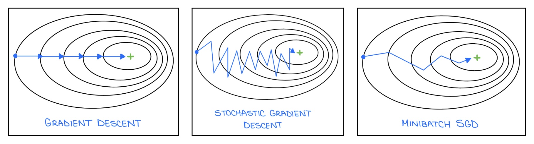
**Figure 6:** Visuals of Gradient Descent, SGD, and Minibatch SGD.
These visualizations highlight the core trade-offs between stability, speed, and computational cost across these optimization strategies.
To summarize: while full-batch gradient descent provides stable and consistent updates, it is computationally expensive. In contrast, SGD and Minibatch SGD offer faster and more scalable updates, but at the cost of increased noise in the optimization path.
#### Behavior in Non-Convex Loss Surfaces
In addition to trade-offs in performance and efficiency, SGD and GD also face challenges that stem from the complex shape of the loss surface, where the optimization landscape is often highly non-convex and filled with irregularities. Common issues include local minima, saddle points, and flat regions.
* __Local Minima:__ Non-convex loss functions naturally contain local minima. Traditional gradient descent can easily get stuck in such points. In contrast, SGD is less likely to get stuck in sharp local minima. This is due to the inherent randomness in its updates: the noise introduced by sampling a single example (or a small batch) allows SGD to "bounce out" of shallow or sharp local minima and contiinue exploring the loss surface.
* __Saddle Points & Flat Regions:__ SGD often slows down or becomes stuck around saddle points or flat regions in the loss surface. For context:
* Saddle points are locations where the gradient is close to zero, but the point is neither a local minimum nor a maximum
* Flat regions, or plateaus, have very small gradients across a wide area, resulting in negligible parameter updates.
In both cases, the optimizer may make very slow progress or fail to converge altogether. To address these challenges, we will turn to techniques like momentum and adaptive optimizers.
#### SGD with Momentum
To improve convergence speed, reduce oscillations, and avoid saddle points, SGD with Momentum introduces a concept called momentum, which accumulates a history of past gradients to smooth out updates. Instead of updating weights directly based on the current gradient, we compute an exponentially weighted moving average (EWMA) of the past gradients. This accumulated value acts like "velocity" in the direction of descent. The udpate rules for SGD with Momentum are:
$$ \mathbf{m}_{t+1} = \mu \ \mathbf{m}_t - \alpha \ \nabla \ell(\mathbf{w}_t, \mathbf{x}_i) $$
$$ \mathbf{w}_{t+1} = \mathbf{w}_t + \mathbf{m}_{t+1} $$
where $ \mu \in [0,1] $ is the momentum coefficient and $ \alpha $ is the learning rate as before.
The momentum term helps the optimizer build speed in consistent descent directions and dampen oscillations in noisy regions. In practice, using momentum almost always leads to faster convergence compared to standard SGD.
### Adaptive Optimizers
In the variants of SGD we covered previously, the same learning rate $ \alpha $ is used for all parameters. But in many cases, especially with sparse data, we want more fine-grained control.
Some features might appear very frequently, while others are rare. We want to take smaller steps (lower learning rates) in directions where the gradient has been consistently large, and larger steps in directions where the gradients are small.
This is the core idea behind adaptive optimizers: learning rates that adapt individually for each parameter.
#### AdaGrad
AdaGrad (short for Adaptive Gradient Algorithm) modifies SGD by assigning individual learning rates to each parameter based on the history of past gradients. It increases learning rates for rarely-updated parameters and decreases them for frequently-updated ones.
The AdaGrad update rule consists of two steps. First, it maintains an accumulator vector $ \mathbf{v}_t $, which stores the sum of squared gradients up to time $ t $:
$$ \mathbf{v}_{t+1} = \mathbf{v}_t + \mathbf{g}_{t}^2 $$
Here, $ \mathbf{g}_t $ is the gradient at time $ t $, and the square is applied element-wise. Second, it updates the weights as follows:
$$ \mathbf{w}_{t+1} = \mathbf{w}_t - \frac{\alpha}{\sqrt{\mathbf{v}_{t+1}+\epsilon}} \ \odot \ \mathbf{g}_t $$
Each component of the gradient vector is scaled by the inverse square root of its accumulated squared gradients, effectively assigning a unique, diminishing learning rate to each parameter.
Although AdaGrad often leads to faster and more stable convergence early in training, one of its key limitations is that the accumulated gradients can grow large over time, causing the learning rates to shrink excessively. This overly aggressive decay can eventually stall learning altogether, especially in longer training runs.
#### RMSProp
Much like momentum, RMSProp (Root Mean Square Propagation) maintains an exponentially weighted moving average of past gradients. Instead of averaging the gradients themselves, however, it simply averages the squared gradients. This technique helps prevent the aggressive learning rate decay that occurs in AdaGrad by giving more weight to recent gradients and gradually "forgetting" older ones. The update rule is as follows:
$$ \mathbf{v}_{t+1} = \beta \mathbf{v}_t + (1-\beta) \ \mathbf{g}_{t}^2 $$
$$ \mathbf{w}_{t+1} = \mathbf{w}_t - \frac{\alpha}{\sqrt{\mathbf{v}_{t+1} + \epsilon}} \ \odot \ \mathbf{g}_t $$
where $ \beta \in [0,1] $ is the exponential moving average constant.
RMSProp adapts the learning rate for each parameter based on the recent magnitude of its gradients, which makes it well-suited for non-stationary objectives, such as those encountered in recurrent neural networks. Compared to AdaGrad, RMSProp generally stabilizes learning and leads to faster, more reliable convergence.
One limitation of RMSProp is that it considers only the magnitude of recent gradients, not their direction. As a result, it cannot accelerate in consistent descent directions. This causes RMSProp to struggle to navigate narrow valleys or curved surfaces efficiently. This is addressed by Adam.
#### Adam
Adam (short for Adaptive Moment Estimation) combines the strength of both momentum and RMSProp into a single, highly effective optimization algorithm. In practice, Adam often outperforms other optimizers and is widely used as the default choice in many deep learning frameworks.
Like momentum, Adam maintains an exponentially weighted decaying average of past gradients to capture the direction of movement. At the same time, like RMSProp, Adam maintains an exponential moving average of squared gradients to adaptively scale the learning rate for each parameter. Adam's update step includes all of the following computations:
* First moment estimate (like momentum): $ \mathbf{m}_{t+1} = \beta_1 \mathbf{m}_t + (1-\beta_1) \ \mathbf{g}_t $
* Second moment estimate (like RMSProp): $ \mathbf{v}_{t+1} = \beta_2 \mathbf{v}_t + (1-\beta_2) \ \mathbf{g}_{t}^2 $
To correct for bias introduced by by initializing $ \mathbf{m}_0 $ and $ \mathbf{v}_0 $ at zero, Adam computes bias-corrected estimates:
$$ \hat{\mathbf{m}}_{t+1} = \frac{\mathbf{m}_{t+1}}{1-\beta_{1}^{t+1}}$$
$$ \hat{\mathbf{v}}_{t+1} = \frac{\mathbf{v}_{t+1}}{1-\beta_{2}^{t+1}} $$
Thus, the weight update becomes
$$ \mathbf{w}_{t+1} = \mathbf{w}_t - \frac{\alpha}{\sqrt{\hat{\mathbf{v}}_{t+1}+\epsilon}} \ \odot \ \hat{\mathbf{m}}_{t+1} $$
Adam is popular because it combines the stability of RMSProp and the acceleration of momentum, often achieving faster convergence and requiring less parameter tuning than SGD.
### Visualization
To build deeper intuition for how different optimization methods behave, you can explore an excellent interactive tool: [Gradient Descent Viz](https://github.com/lilipads/gradient_descent_viz/tree/master?tab=readme-ov-file).
This desktop application visualizes several popular optimization algorithms, including: Gradient Descent, Momentum, AdaGrad, RMSProp, and Adam. You can experiment with learning rates, momentum values, and other hyperparameters to see how they affect convergence and path trajectories.
In addition to the interactive app, the following two GIFs offer helpful visual comparisons that highlight how various optimizers behave side by side in different optimization scenarios.
**Figure 5:** Dependency graph for the final layer $ L $ of our MLP.
Hence, the general form of the chain rule tells us that
$$ \frac{\partial \mathcal{L}}{\partial \mathbf{W}^{[L]}}=\frac{\partial \mathcal{L}}{\partial \mathbf{z}^{[L]}} \frac{\partial \mathbf{z}^{[L]}}{\partial \mathbf{a}^{[L]}} \frac{\partial \mathbf{a}^{[L]}}{\partial \mathbf{W}^{[L]}} \ \text{ and } \ \frac{\partial \mathcal{L}}{\partial \mathbf{b}^{[L]}}=\frac{\partial \mathcal{L}}{\partial \mathbf{z}^{[L]}} \frac{\partial \mathbf{z}^{[L]}}{\partial \mathbf{a}^{[L]}} \frac{\partial \mathbf{a}^{[L]}}{\partial \mathbf{b}^{[L]}} $$
We see that $$ \frac{\partial \mathcal{L}}{\partial \mathbf{a}^{[L]}} = \frac{\partial \mathcal{L}}{\partial \mathbf{z}^{[L]}} \frac{\partial \mathbf{z}^{[L]}}{\partial \mathbf{a}^{[L]}} $$
appears in our expressions for $ \frac{\partial \mathcal{L}}{\partial \mathbf{W}^{[L]}} $ and $ \frac{\partial \mathcal{L}}{\partial \mathbf{b}^{[L]}} $, so we compute $ \frac{\partial \mathcal{L}}{\partial \mathbf{a}^{[L]}} = \delta^{[L]} $ first.
#### Line 2: Computing $ \delta^{[L]} $
Using the chain rule from Equation (1), we have
$$ \delta^{[L]}= \frac{\partial \mathcal{L}}{\partial \mathbf{a}^{[L]}} = \left(\frac{\partial \mathbf{z}^{[L]}}{\partial \mathbf{a}^{[L]}} \right)^T \frac{\partial \mathcal{L}}{\partial \mathbf{z}^{[L]}}$$
where $ \delta^{[L]} $ is shorthand for $ \frac{\partial \mathcal{L}}{\partial \mathbf{a}^{[L]}} $.
>**Remark:** Although the final output of the network is typically a scalar, we treat $ \mathbf{z}^{[L]} $ as a (1-dimensional) vector so that the same derivation applies to all layers $ l \in \{1, 2, ..., L-1\} $, where $ \mathbf{z}^{[l]} $ is vector-valued.
We can compute $ \frac{\partial \mathcal{L}}{\partial \mathbf{z}^{[L]}} $ directly. What remains is to compute $ \frac{\partial \mathbf{z}^{[L]}}{\partial \mathbf{a}^{[L]}} $.
Since $ \mathbf{z}^{[L]} = \sigma(\mathbf{a}^{[L]}) $ and $ \mathbf{z}^{[L]}, \mathbf{a}^{[L]} \in \mathbb{R}^n $, the Jacobian is
$$ \frac{\partial \mathbf{z}^{[L]}}{\partial \mathbf{a}^{[L]}} = \begin{bmatrix} \frac{\partial}{\partial a_1^{[L]}} \left[\sigma(a_1^{[L]}) \right] & \ldots & \frac{\partial}{\partial a_n^{[L]}} \left[ \sigma(a_1^{[L]})\right] \\ \vdots & \ddots & \vdots \\ \frac{\partial}{\partial a_1^{[L]}} \left[\sigma(a_n^{[L]})\right] & \ldots & \frac{\partial}{\partial a_n^{[L]}} \left[ \sigma(a_n^{[L]}) \right]\end{bmatrix} = \begin{bmatrix} \sigma'(a_1^{[L]}) & \ldots & 0 \\ \vdots & \ddots & \vdots \\ 0 & \ldots & \sigma'(a_n^{[L]})\end{bmatrix}$$
(a diagonal matrix), which gives us
$$ \left(\frac{\partial \mathbf{z}^{[L]}}{\partial \mathbf{a}^{[L]}} \right)^T \frac{\partial \mathcal{L}}{\partial \mathbf{z}^{[L]}} = \begin{bmatrix} \sigma'(a_1^{[L]}) & \ldots & 0 \\ \vdots & \ddots & \vdots \\ 0 & \ldots & \sigma'(a_n^{[L]})\end{bmatrix} \begin{bmatrix} \frac{\partial \mathcal{L}}{\partial z_1^{[L]}} \\ \vdots \\ \frac{\partial \mathcal{L}}{\partial z_n^{[L]}} \end{bmatrix} = \begin{bmatrix} \frac{\partial \mathcal{L}}{\partial z_1^{[L]}} \cdot \sigma'(a_1^{[L]}) \\ \vdots \\ \frac{\partial \mathcal{L}}{\partial z_n^{[L]}} \cdot \sigma'(a_n^{[L]}) \end{bmatrix} $$
We can rewrite the above using $ \odot $, the symbol for element-wise multiplication, to conclude
$$ \frac{\partial \mathcal{L}}{\partial \mathbf{a}^{[L]}} = \frac{\partial \mathcal{L}}{\partial \mathbf{z}^{[L]}} \odot \sigma'(\mathbf{a}^{[L]}) $$
as expected.
#### Line 4: Computing $ \frac{\partial \mathcal{L}}{\partial \mathbf{W}^{[L]}} $
We have that
$$ \frac{\partial \mathcal{L}}{\partial \mathbf{W}^{[L]}} = \frac{\partial \mathcal{L}}{\partial \mathbf{a}^{[L]}} \frac{\partial \mathbf{a}^{[L]}}{\partial \mathbf{W}^{[L]}} $$
We will not use Equation (1) directly, since we are differentiating with respect to a matrix $ \mathbf{W}^{[L]} \in \mathbb{R}^{n \times m} $ rather than a vector.
>If we flattened $ \mathbf{W}^{[L]} \in \mathbb{R}^{n \times m} $ to an $ nm $-dimensional column vector and used Equation (1), we would get $ \frac{\partial \mathcal{L}}{\partial \mathbf{W}^{[L]}} = \left(\frac{\partial \mathbf{a}^{[L]}}{\partial \mathbf{W}^{[L]}} \right)^T \frac{\partial \mathcal{L}}{\partial \mathbf{a}^{[L]}} $ where the Jacobian $ \frac{\partial \mathbf{a}^{[L]}}{\partial \mathbf{W}^{[L]}} \in \mathbb{R}^{n \times nm} $. This implies $ \frac{\partial \mathcal{L}}{\partial \mathbf{W}^{[L]}} \in \mathbb{R}^{nm} $ would be an $ nm $-dimensonal column vector, which does not match the shape of $ \mathbf{W}^{[L]} \in \mathbb{R}^{n \times m} $ (and, at least in theory, we want these shapes to align).
We would like $ \frac{\partial \mathcal{L}}{\partial \mathbf{W}^{[L]}} $ to also be an $ n \times m $ matrix of the form
$$\frac{\partial \mathcal{L}}{\partial \mathbf{W}^{[L]}} = \begin{bmatrix} \frac{\partial \mathcal{L}}{\partial W_{11}^{[L]}} & \ldots & \frac{\partial \mathcal{L}}{\partial W_{1m}^{[L]}} \\ \vdots & \ddots & \vdots \\ \frac{\partial \mathcal{L}}{\partial W_{n1}^{[L]}} & \ldots & \frac{\partial \mathcal{L}}{\partial W_{nm}^{[L]}} \end{bmatrix}$$
Consider the $ (i,j) $ entry of $ \frac{\partial \mathcal{L}}{\partial \mathbf{W}^{[L]}} $. By the general form of the chain rule,
$$ \frac{\partial \mathcal{L}}{\partial W_{ij}^{[L]}} = \frac{\partial \mathcal{L}}{\partial a_i^{[L]}} \frac{\partial a_i^{[L]}}{\partial W_{ij}^{[L]}} $$
(which we can do because $ a_i $ is the only component of $ \mathbf{a}^{[L]} $ that uses $ W_{ij}^{[L]} $ in its computation). Note that $ \frac{\partial \mathcal{L}}{\partial a_i^{[L]}} $ is the $ i $-th entry of $ \delta^{[L]} $ by definition. Furthermore, observe that
$$ \frac{\partial a_i^{[L]}}{\partial W_{ij}^{[L]}} = \frac{\partial}{\partial W_{ij}^{[L]}} \left[\left(\sum_{k=1}^m W_{ik}^{[L]} z_k^{[L-1]}\right) + b_i^{[L]} \right] = z_j^{[L-1]} $$
Thus, the $ (i,j) $ entry of $ \frac{\partial \mathcal{L}}{\partial \mathbf{W}^{[L]}} $ is given by
$$ \frac{\partial \mathcal{L}}{\partial W_{ij}^{[L]}} = \delta_i^{[L]} z_j^{[L-1]} $$
meaning $ \frac{\partial \mathcal{L}}{\partial \mathbf{W}^{[L]}} $ is equal to the outer product
$$ \frac{\partial \mathcal{L}}{\partial \mathbf{W}^{[L]}} = \delta^{[L]} \left(\mathbf{z}^{[L-1]}\right)^T $$
as expected. (We can confirm that multiplying $ \delta^{[L]} \in \mathbb{R}^{n \times 1} $ and $ (\mathbf{z}^{[L-1]})^T \in \mathbb{R}^{1\times m} $ does indeed yield an $ n \times m $ matrix.)
>**Remark:** This section was from [Computing Neural Network Gradients](https://web.stanford.edu/class/archive/cs/cs224n/cs224n.1184/readings/gradient-notes.pdf) (Kevin Clark, Stanford), which offers another explanation of how to derive $ \frac{\partial \mathcal{L}}{\partial \mathbf{W}^{[L]}} $ on p.3.
#### Line 5: Computing $ \frac{\partial \mathcal{L}}{\partial \mathbf{b}^{[L]}} $
Using the chain rule from Equation (1), we have
$$ \frac{\partial \mathcal{L}}{\partial \mathbf{b}^{[L]}} = \left( \frac{\partial \mathbf{a}^{[L]}}{\partial \mathbf{b}^{[L]}} \right)^T \frac{\partial \mathcal{L}}{\partial \mathbf{a}^{[L]}} $$
We already computed $ \frac{\partial \mathcal{L}}{\partial \mathbf{a}^{[L]}}=\delta^{[L]} $, so we need $ \frac{\partial \mathbf{a}^{[L]}}{\partial \mathbf{b}^{[L]}} $. Since $ \mathbf{a}^{[L]}, \mathbf{b}^{[L]} \in \mathbb{R}^n $, the Jacobian is
$$ \frac{\partial \mathbf{a}^{[L]}}{\partial \mathbf{b}^{[L]}} = \begin{bmatrix} \frac{\partial a_1^{[L]}}{\partial b_1^{[L]}} & \ldots & \frac{\partial a_1^{[L]}}{\partial b_n^{[L]}} \\ \vdots & \ddots & \vdots \\ \frac{\partial a_n^{[L]}}{\partial b_1^{[L]}} & \ldots & \frac{\partial a_n^{[L]}}{\partial b_n^{[L]}} \end{bmatrix} $$
Consider the $ (1,1) $ entry:
$$ \frac{\partial a_1^{[L]}}{\partial b_1^{[L]}} = \frac{\partial}{\partial b_1^{[L]}} \left[ \left(\sum_{j=1}^m W_{1j}^{[L]}z_j^{[L-1]} \right)+ b_1^{[L]}\right] = 1 $$
More generally,
$$\frac{\partial a_i^{[L]}}{\partial b_j^{[L]}}=\begin{cases} 1 & \text{if } i=j \\ 0 & \text{otherwise} \end{cases} \ \Rightarrow \ \frac{\partial \mathbf{a}^{[L]}}{\partial \mathbf{b}^{[L]}} = I_{n \times n}\ $$
so we conclude that
$$ \frac{\partial \mathcal{L}}{\partial \mathbf{b}^{[L]}} = \delta^{[L]} $$
as expected.
#### Line 6: Computing $ \frac{\partial \mathcal{L}}{\partial \mathbf{z}^{[L-1]}} $
>**Why are we computing $ \frac{\partial \mathcal{L}}{\partial \mathbf{z}^{[L-1]}} $?**
If we look ahead to Line 7 in the backpropagation algorithm, we need $ \frac{\partial \mathcal{L}}{\partial \mathbf{z}^{[L-1]}} $ in order to compute $ \delta^{[L-1]} $, which will be key for computing the gradients of the loss with respect to the weights and biases of layer $ L-1 $.
Using the chain rule from Equation (1),
$$ \frac{\partial \mathcal{L}}{\partial \mathbf{z}^{[L-1]}} = \left(\frac{\partial \mathbf{a}^{[L]}}{\partial \mathbf{z}^{[L-1]}} \right)^T \frac{\partial \mathcal{L}}{\partial \mathbf{a}^{[L]}} $$
We already computed $ \frac{\partial \mathcal{L}}{\partial \mathbf{a}^{[L]}}=\delta^{[L]} $, so we need $ \frac{\partial \mathbf{a}^{[L]}}{\partial \mathbf{z}^{[L-1]}} $. Since $ \mathbf{a}^{[L]} \in \mathbb{R}^n $ and $ \mathbf{z}^{[L-1]} \in \mathbb{R}^m $, the Jacobian is
$$ \frac{\partial \mathbf{a}^{[L]}}{\partial \mathbf{z}^{[L-1]}} = \begin{bmatrix} \frac{\partial a_1^{[L]}}{\partial z_1^{[L-1]}} & \ldots & \frac{\partial a_1^{[L]}}{\partial z_m^{[L-1]}} \\ \vdots & \ddots & \vdots \\ \frac{\partial a_n^{[L]}}{\partial z_1^{[L-1]}} & \ldots & \frac{\partial a_n^{[L]}}{\partial z_m^{[L-1]}} \end{bmatrix} $$
Consider the $ (n,1) $ entry:
$$ \frac{\partial a_n^{[L]}}{\partial z_1^{[L-1]}} = \frac{\partial}{\partial z_1^{[L-1]}} \left[\left(\sum_{j=1}^m W_{nj}z_j^{[L-1]}\right) + b_n^{[L]} \right] = W_{n1}^{[L]} $$
(since the $ a_n^{[L]} $ entry of $ \mathbf{a}^{[L]} $ is given by dotting the $ n^{\text{th}} $ row of $ \mathbf{W}^{[L]} $ with $ \mathbf{z}^{[L-1]} $ and adding the last entry $ b_n^{[L]} $ of the bias). In general, the $ (i,j) $ entry of $ \frac{\partial \mathbf{a}^{[L]}}{\partial \mathbf{z}^{[L-1]}} $ is given by
$$ \frac{\partial a_i^{[L]}}{\partial z_j^{[L-1]}} = W_{ij}^{[L]} \ \Rightarrow \ \frac{\partial \mathbf{a}^{[L]}}{\partial \mathbf{z}^{[L-1]}} = \mathbf{W}^{[L]}$$
Thus, we conclude
$$ \frac{\partial \mathcal{L}}{\partial \mathbf{z}^{[L-1]}} = \left(\mathbf{W}^{[L]}\right)^T \delta^{[L]} $$
as expected.
#### Line 7: Computing $ \delta^{[L-1]} $
Just as we used $ \delta^{[L]} $ to compute $ \frac{\partial \mathcal{L}}{\partial \mathbf{W}^{[L]}} $ and $ \frac{\partial \mathcal{L}}{\partial \mathbf{b}^{[L]}} $, we want $ \delta^{[L-1]} $ so that we can obtain $ \frac{\partial \mathcal{L}}{\partial \mathbf{W}^{[L-1]}} $ and $ \frac{\partial \mathcal{L}}{\partial \mathbf{b}^{[L-1]}} $. From identical logic to Line 2, we have
$$ \delta^{[L-1]} = \frac{\partial \mathcal{L}}{\partial \mathbf{z}^{[L-1]}} \odot \sigma'(\mathbf{a}^{[L-1]}) $$
Using our work from Line 6 and taking $ \mathbf{a}^{[L-1]} $ from the forward pass, we can compute
$$ \delta^{[L-1]} = \left(\left(\mathbf{W}^{[L]}\right)^T \delta^{[L]} \right) \odot \sigma'(\mathbf{a}^{[L-1]}) $$
and begin our computation of $ \frac{\partial \mathcal{L}}{\partial \mathbf{W}^{[L-1]}} $ and $ \frac{\partial \mathcal{L}}{\partial \mathbf{b}^{[L-1]}} $. We keep repeating this loop, propagating gradients back through the network, until we have $ \frac{\partial \mathcal{L}}{\partial \mathbf{W}^{[l]}} $ and $ \frac{\partial \mathcal{L}}{\partial \mathbf{b}^{[l]}} $ for $ l \in \{1, 2, ..., L-1\} $ as well. Our final output is all of these gradients:
$$ \frac{\partial \mathcal{L}}{\partial \mathbf{W}^{[1:L]}} \text{ and } \frac{\partial \mathcal{L}}{\partial \mathbf{b}^{[1:L]}}$$
which we pass to our chosen optimizer!
### Update Step
Now that we have all of these gradients, how do we actually change the weights and bias terms? The update step depends on our optimization algorithm (see the "Optimization" section for a detailed description of the tradeoffs between different optimization algorithms). If we are just using vanilla gradient descent (GD) on a training dataset $ \mathcal{D}_{TR}=\{\mathbf{x_i},\mathbf{y_i}\}_{i=0}^n $, the update step looks like the following:
$$ \mathbf{w}_{t+1}= \mathbf{w}_t-\alpha \nabla\mathcal{L}(\mathbf{w_t; \mathcal{D}_{TR}}) $$
where $ \alpha $ is our learning rate and the gradient of the loss function $ \nabla\mathcal{L}(\mathbf{w_t}) $ is the gradient over all training points:
$$ \nabla\mathcal{L}(\mathbf{w}_t; \mathcal{D}_{TR})=\frac{1}{n} \sum_{i}^n \nabla \ell(\mathbf{w_t}, \mathbf{x}_i) $$
Again, see below for other (far better) optimization algorithms. Regardless of which optimizer we use, though, after we have updated our weights, we are ready for the next forward pass!
__Sources__:
* [Multi-Layer Perceptron Learning in Tensorflow](https://www.geeksforgeeks.org/multi-layer-perceptron-learning-in-tensorflow/) (GeeksforGeeks)
* [Recap & Multi-Layer Perceptrons Slides](https://www.cs.cornell.edu/courses/cs4782/2025sp/slides/pdf/week1_2_slides_complete.pdf) (CS 4/5782: Deep Learning, Spring 2025)
* [Mastering Tanh: A Deep Dive into Balanced Activation for Machine Learning](https://medium.com/ai-enthusiast/mastering-tanh-a-deep-dive-into-balanced-activation-for-machine-learning-4734ec147dd9) (Medium)
* [Exploring the Power and Limitations of Multi-Layer Perceptron (MLP) in Machine Learning](https://shekhar-banerjee96.medium.com/exploring-the-power-and-limitations-of-multi-layer-perceptron-mlp-in-machine-learning-d97a3f84f9f4) (Medium)
## Optimization
In deep learning, improving a model involves minimizing the difference between its predictions and the true labels (i.e., minimizing how far the model's predictions are from the actual values). This difference is quantified using a loss function.
Let us use $ \ell(\mathbf{w}_t, \mathbf{x}_i) $ to define the per-sample loss at time step $ t $, where $ \mathbf{w}_t $ are the model weights at time $ t $ and $ \mathbf{x}_i $ is a data point. The overall objective is to minimize the empirical risk, i.e., the average loss across the dataset, which, as above can be defined as:
$$ \mathcal{L}(\mathbf{w}_t;\mathcal{D}_{TR})= \frac{1}{n} \sum_{i}^n \ \ell(\mathbf{w}_t, \mathbf{x}_i) $$
The goal of optimization algorithms is to find the model weights $ \mathbf{w} $ that minimize this loss function. Broadly, optimizers can be categorized into two types:
1. __Non-Adaptive Optimizers:__ Use the same learning rate for all parameters. Examples include: Gradient Descent (GD), Stochastic Gradient Descent (SGD), Minibatch SGD, and SGD with Momentum.
2. __Adaptive Optimizers:__ Adjust the learning rate for each parameter individually based on past gradients. Examples include: AdaGrad, RMSProp, and Adam.
We will explore both non-adaptive and adaptive optimization methods in detail below.
### Non-Adaptive Optimizers
#### Gradient Descent
Gradient descent is the foundational optimization method that the other, more advanced optimizers build on. At each step, the model's parameters are updated in the direction that reduces the loss the most: since the gradient points in the direction of steepest *ascent* over the loss surface, we want to move in the opposite direction ($ \Rightarrow $ negation) of the gradient.
The standard update rule for the traditional gradient descent algorithm is
$$ \mathbf{w}_{t+1} = \mathbf{w}_t - \alpha \nabla\mathcal{L}(\mathbf{w}_t) $$
where $ \mathbf{w}_t $ are the weights at time $ t $, $ \alpha $ is the learning rate, and $ \nabla\mathcal{L}(\mathbf{w}_t)=\frac{1}{n}\sum_i^n \nabla \ell(\mathbf{w}_t,\mathbf{x}_i) $ is the average gradient over the dataset.
__Key Limitation__: Each update step requires computing the gradient across all training data points. For large datasets, this is computationally expensive, slow, and memory-intensive, making standard gradient descent inefficient in practice (especially when fast updates are desired).
#### Stochastic Gradient Descent (SGD)
Stochastic Gradient Descent addresses the inefficiency of full-batch (or traditional) gradient descent by computing the gradient using only one randomly selected sample at each iteration. As a result, the update rule for SGD is:
$$ \mathbf{w}_{t+1} = \mathbf{w}_t - \alpha \ \nabla \ell(\mathbf{w}_t, \mathbf{x}_i) $$
While this approach is much faster per iteration and suitable for large datasets, it introduces a new challenge: the gradients from individual samples are often noisy and do not necessarily point toward the direction of the true minimum. This may cause the optimization path to fluctuate significantly, introducing a "noise ball" effect where updates wander before settling near a minimum.
Despite this, stochastic gradients are unbiased estimates of the true gradient; in expectation, the per-sample gradient is equivalent to the full gradient:
$$ \mathbb{E} [\nabla \ell(\mathbf{w}_t, \mathbf{x}_i)] = \nabla \mathcal{L}(\mathbf{w}_t) $$
This means that, with appropriate tuning of the learning rate, SGD can still converge effectively in practice.
#### Minibatch SGD
Minibatch SGD strikes a balance between the extremes of full gradient descent and pure SGD. Instead of computing the gradient over all data or a single sample, it does so over a randomly selected batch of samples $ \mathcal{B}_t $ with batch size $ b $. The update rule then becomes
$$ \mathbf{w}_{t+1} = \mathbf{w}_t - \alpha \cdot \frac{1}{b} \sum_{i \in \mathcal{B}_t} \nabla \ell(\mathbf{w}_t, \mathbf{x}_i) $$
This approach benefits from reduced noise compared to pure SGD due to averaging over multiple samples, while still being significantly faster and more memory-efficient than full-batch gradient descent. However, minibatch SGD still involves some noise and does not provide as smooth a convergence path as full gradient descent.
Let us now visualize how different optimization strategies traverse the loss surface. The figure below compares Gradient Descent, Stochastic Gradient Descent, and Minibatch SGD in terms of their update trajectories:

**Figure 6:** Visuals of Gradient Descent, SGD, and Minibatch SGD.
These visualizations highlight the core trade-offs between stability, speed, and computational cost across these optimization strategies.
To summarize: while full-batch gradient descent provides stable and consistent updates, it is computationally expensive. In contrast, SGD and Minibatch SGD offer faster and more scalable updates, but at the cost of increased noise in the optimization path.
#### Behavior in Non-Convex Loss Surfaces
In addition to trade-offs in performance and efficiency, SGD and GD also face challenges that stem from the complex shape of the loss surface, where the optimization landscape is often highly non-convex and filled with irregularities. Common issues include local minima, saddle points, and flat regions.
* __Local Minima:__ Non-convex loss functions naturally contain local minima. Traditional gradient descent can easily get stuck in such points. In contrast, SGD is less likely to get stuck in sharp local minima. This is due to the inherent randomness in its updates: the noise introduced by sampling a single example (or a small batch) allows SGD to "bounce out" of shallow or sharp local minima and contiinue exploring the loss surface.
* __Saddle Points & Flat Regions:__ SGD often slows down or becomes stuck around saddle points or flat regions in the loss surface. For context:
* Saddle points are locations where the gradient is close to zero, but the point is neither a local minimum nor a maximum
* Flat regions, or plateaus, have very small gradients across a wide area, resulting in negligible parameter updates.
In both cases, the optimizer may make very slow progress or fail to converge altogether. To address these challenges, we will turn to techniques like momentum and adaptive optimizers.
#### SGD with Momentum
To improve convergence speed, reduce oscillations, and avoid saddle points, SGD with Momentum introduces a concept called momentum, which accumulates a history of past gradients to smooth out updates. Instead of updating weights directly based on the current gradient, we compute an exponentially weighted moving average (EWMA) of the past gradients. This accumulated value acts like "velocity" in the direction of descent. The udpate rules for SGD with Momentum are:
$$ \mathbf{m}_{t+1} = \mu \ \mathbf{m}_t - \alpha \ \nabla \ell(\mathbf{w}_t, \mathbf{x}_i) $$
$$ \mathbf{w}_{t+1} = \mathbf{w}_t + \mathbf{m}_{t+1} $$
where $ \mu \in [0,1] $ is the momentum coefficient and $ \alpha $ is the learning rate as before.
The momentum term helps the optimizer build speed in consistent descent directions and dampen oscillations in noisy regions. In practice, using momentum almost always leads to faster convergence compared to standard SGD.
### Adaptive Optimizers
In the variants of SGD we covered previously, the same learning rate $ \alpha $ is used for all parameters. But in many cases, especially with sparse data, we want more fine-grained control.
Some features might appear very frequently, while others are rare. We want to take smaller steps (lower learning rates) in directions where the gradient has been consistently large, and larger steps in directions where the gradients are small.
This is the core idea behind adaptive optimizers: learning rates that adapt individually for each parameter.
#### AdaGrad
AdaGrad (short for Adaptive Gradient Algorithm) modifies SGD by assigning individual learning rates to each parameter based on the history of past gradients. It increases learning rates for rarely-updated parameters and decreases them for frequently-updated ones.
The AdaGrad update rule consists of two steps. First, it maintains an accumulator vector $ \mathbf{v}_t $, which stores the sum of squared gradients up to time $ t $:
$$ \mathbf{v}_{t+1} = \mathbf{v}_t + \mathbf{g}_{t}^2 $$
Here, $ \mathbf{g}_t $ is the gradient at time $ t $, and the square is applied element-wise. Second, it updates the weights as follows:
$$ \mathbf{w}_{t+1} = \mathbf{w}_t - \frac{\alpha}{\sqrt{\mathbf{v}_{t+1}+\epsilon}} \ \odot \ \mathbf{g}_t $$
Each component of the gradient vector is scaled by the inverse square root of its accumulated squared gradients, effectively assigning a unique, diminishing learning rate to each parameter.
Although AdaGrad often leads to faster and more stable convergence early in training, one of its key limitations is that the accumulated gradients can grow large over time, causing the learning rates to shrink excessively. This overly aggressive decay can eventually stall learning altogether, especially in longer training runs.
#### RMSProp
Much like momentum, RMSProp (Root Mean Square Propagation) maintains an exponentially weighted moving average of past gradients. Instead of averaging the gradients themselves, however, it simply averages the squared gradients. This technique helps prevent the aggressive learning rate decay that occurs in AdaGrad by giving more weight to recent gradients and gradually "forgetting" older ones. The update rule is as follows:
$$ \mathbf{v}_{t+1} = \beta \mathbf{v}_t + (1-\beta) \ \mathbf{g}_{t}^2 $$
$$ \mathbf{w}_{t+1} = \mathbf{w}_t - \frac{\alpha}{\sqrt{\mathbf{v}_{t+1} + \epsilon}} \ \odot \ \mathbf{g}_t $$
where $ \beta \in [0,1] $ is the exponential moving average constant.
RMSProp adapts the learning rate for each parameter based on the recent magnitude of its gradients, which makes it well-suited for non-stationary objectives, such as those encountered in recurrent neural networks. Compared to AdaGrad, RMSProp generally stabilizes learning and leads to faster, more reliable convergence.
One limitation of RMSProp is that it considers only the magnitude of recent gradients, not their direction. As a result, it cannot accelerate in consistent descent directions. This causes RMSProp to struggle to navigate narrow valleys or curved surfaces efficiently. This is addressed by Adam.
#### Adam
Adam (short for Adaptive Moment Estimation) combines the strength of both momentum and RMSProp into a single, highly effective optimization algorithm. In practice, Adam often outperforms other optimizers and is widely used as the default choice in many deep learning frameworks.
Like momentum, Adam maintains an exponentially weighted decaying average of past gradients to capture the direction of movement. At the same time, like RMSProp, Adam maintains an exponential moving average of squared gradients to adaptively scale the learning rate for each parameter. Adam's update step includes all of the following computations:
* First moment estimate (like momentum): $ \mathbf{m}_{t+1} = \beta_1 \mathbf{m}_t + (1-\beta_1) \ \mathbf{g}_t $
* Second moment estimate (like RMSProp): $ \mathbf{v}_{t+1} = \beta_2 \mathbf{v}_t + (1-\beta_2) \ \mathbf{g}_{t}^2 $
To correct for bias introduced by by initializing $ \mathbf{m}_0 $ and $ \mathbf{v}_0 $ at zero, Adam computes bias-corrected estimates:
$$ \hat{\mathbf{m}}_{t+1} = \frac{\mathbf{m}_{t+1}}{1-\beta_{1}^{t+1}}$$
$$ \hat{\mathbf{v}}_{t+1} = \frac{\mathbf{v}_{t+1}}{1-\beta_{2}^{t+1}} $$
Thus, the weight update becomes
$$ \mathbf{w}_{t+1} = \mathbf{w}_t - \frac{\alpha}{\sqrt{\hat{\mathbf{v}}_{t+1}+\epsilon}} \ \odot \ \hat{\mathbf{m}}_{t+1} $$
Adam is popular because it combines the stability of RMSProp and the acceleration of momentum, often achieving faster convergence and requiring less parameter tuning than SGD.
### Visualization
To build deeper intuition for how different optimization methods behave, you can explore an excellent interactive tool: [Gradient Descent Viz](https://github.com/lilipads/gradient_descent_viz/tree/master?tab=readme-ov-file).
This desktop application visualizes several popular optimization algorithms, including: Gradient Descent, Momentum, AdaGrad, RMSProp, and Adam. You can experiment with learning rates, momentum values, and other hyperparameters to see how they affect convergence and path trajectories.
In addition to the interactive app, the following two GIFs offer helpful visual comparisons that highlight how various optimizers behave side by side in different optimization scenarios.
 **Figure 7:** Optimization Graphic 1 ([Complete Guide to Adam Optimization, Medium](https://medium.com/@LayanSA/complete-guide-to-adam-optimization-1e5f29532c3d))
In this first GIF, we clearly observe that Adam and RMSProp converge at a similar and notably faster rate than the others, quickly navigating toward the minimum. In contrast, AdaGrad seems to struggle with convergence, reflecting its tendency to decay learning rates too aggressively over time.
**Figure 7:** Optimization Graphic 1 ([Complete Guide to Adam Optimization, Medium](https://medium.com/@LayanSA/complete-guide-to-adam-optimization-1e5f29532c3d))
In this first GIF, we clearly observe that Adam and RMSProp converge at a similar and notably faster rate than the others, quickly navigating toward the minimum. In contrast, AdaGrad seems to struggle with convergence, reflecting its tendency to decay learning rates too aggressively over time.
 **Figure 8:** Optimization Graphic 2 ([Complete Guide to Adam Optimization, Medium](https://medium.com/@LayanSA/complete-guide-to-adam-optimization-1e5f29532c3d))
In this second GIF, we can observe that SGD, AdaGrad, and RMSProp are all taking a similar path, but AdaGrad adn RMSProp are clearly faster. This shows the advantage of using adaptive learning rates. Additionally, we can see that momentum explores a wider region of loss surface initially before taking the direct path to the minimum. This capacity allows it to escape early traps like saddle points.
**Sources:**
* [Optimization Slides](https://www.cs.cornell.edu/courses/cs4782/2025sp/slides/pdf/week2_1_slides_complete.pdf) (CS 4/5782: Deep Learning, Spring 2025)
* [Complete Guide to Adam Optimization](https://medium.com/@LayanSA/complete-guide-to-adam-optimization-1e5f29532c3d) (Medium)
* [ML | Stochastic Gradient Descent (SGD)](https://www.geeksforgeeks.org/ml-stochastic-gradient-descent-sgd/) (GeeksforGeeks)
**Figure 8:** Optimization Graphic 2 ([Complete Guide to Adam Optimization, Medium](https://medium.com/@LayanSA/complete-guide-to-adam-optimization-1e5f29532c3d))
In this second GIF, we can observe that SGD, AdaGrad, and RMSProp are all taking a similar path, but AdaGrad adn RMSProp are clearly faster. This shows the advantage of using adaptive learning rates. Additionally, we can see that momentum explores a wider region of loss surface initially before taking the direct path to the minimum. This capacity allows it to escape early traps like saddle points.
**Sources:**
* [Optimization Slides](https://www.cs.cornell.edu/courses/cs4782/2025sp/slides/pdf/week2_1_slides_complete.pdf) (CS 4/5782: Deep Learning, Spring 2025)
* [Complete Guide to Adam Optimization](https://medium.com/@LayanSA/complete-guide-to-adam-optimization-1e5f29532c3d) (Medium)
* [ML | Stochastic Gradient Descent (SGD)](https://www.geeksforgeeks.org/ml-stochastic-gradient-descent-sgd/) (GeeksforGeeks)