# Regularization
## Motivation
Complex models like deep neural networks can overfit to the training data, meaning they learn patterns—including noise—too specifically and fail to generalize to new data. This generalization gap means that test error could be very high even though training error is low.
Regularization refers to techniques that help prevent overfitting, aiming to minimize the true loss. Regularization adds a preference for *simpler models or solutions*, which tend to generalize better to unseen data.
This relates to a concept known as the Bias-Variance Tradeoff, a fundamental idea in statistical learning theory. Model performance typically follows a U-shaped curve: as model complexity increases, the total error initially decreases but then rises again due to overfitting.
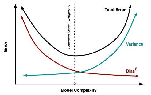 **Figure 1:** Variation of Bias and Variance with model complexity; more complex models overfit, while the simplest models underfit [Scott Fortmann-Roe, 2012](https://scott.fortmann-roe.com/docs/BiasVariance.html)
As we will see later, this is not the full picture for deep networks: with the phenomenon of deep double descent, sometimes the test error decreases again after the point of overfitting. In general, though, regularization encapsulates helpful ways to reduce overfitting and improve generalization of deep learning models.
## Early Stopping
Early stopping is a regularization technique that works by monitoring the performance of a model on the validation set during the training phase. Instead of training a model until the training error converges, early stopping halts the training loop when the validation error ceases to improve.
**Figure 1:** Variation of Bias and Variance with model complexity; more complex models overfit, while the simplest models underfit [Scott Fortmann-Roe, 2012](https://scott.fortmann-roe.com/docs/BiasVariance.html)
As we will see later, this is not the full picture for deep networks: with the phenomenon of deep double descent, sometimes the test error decreases again after the point of overfitting. In general, though, regularization encapsulates helpful ways to reduce overfitting and improve generalization of deep learning models.
## Early Stopping
Early stopping is a regularization technique that works by monitoring the performance of a model on the validation set during the training phase. Instead of training a model until the training error converges, early stopping halts the training loop when the validation error ceases to improve.
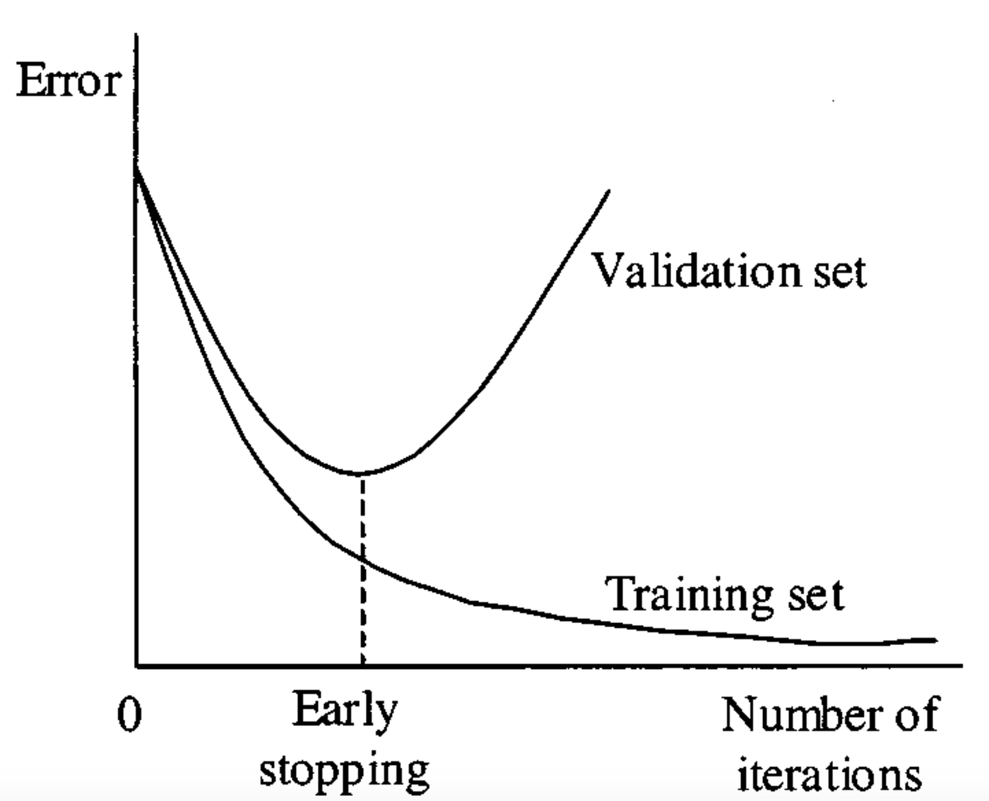 **Figure 2:** Early stopping illustration ([Medium, 2024](https://miro.medium.com/v2/resize:fit:1400/1*-37i5H3lie_x5299utHX4A.png))
The parabolic shape of the validation error gives a good visual for the overfitting risk that arises when training until convergence. Should the model become too "familiar" with the training set, we see overfitting occur, and thus worse generalization. Early stopping aims to avoid this phenomenon by halting training at the point where the model "best" generalizes to some set of unseen data.
## L1 and L2 Regularization
Both $ L1 $ and $ L2 $ regularization add a penalty for complex weights $ \mathbf{w} $ to the optimization problem. The classic goal of Empirical Risk Minimization (ERM) is to find the set of weights $ \mathbf{w} $ that minimizes error over a training dataset $ \mathcal{D}_{TR}=\{\mathbf{x_i},\mathbf{y_i}\}_{i=0}^n $, which we formulate as the following optimization problem:
$$ \textbf{w} = \operatorname{argmin}_{\mathbf{w}} \ \mathcal{L}(\mathbf{w}; \mathcal{D}_{TR})=\operatorname{argmin}_{\mathbf{w}} \frac{1}{n} \sum_i^n \ell(\mathbf{\hat{y}}_i, \mathbf{y}_i) $$
In *Regularized* Empirical Risk Minimization, we want to find a set of weights $ \mathbf{w} $ that minimizes training loss (as before) while also avoiding a complex ($ \Rightarrow $ overfit) solution, giving us the following optimization problem:
$$ \textbf{w} = \operatorname{argmin}_{\mathbf{w}} \ \mathcal{L}(\mathbf{w};\mathcal{D}_{TR})+\lambda \cdot r(\mathbf{w})$$
where $ r(\mathbf{w}) $ measures the complexity of the model (e.g., via $ L1 $ or $ L2 $ norms) and $ \lambda \in \mathbb{R} $ is a hyperparameter that controls the strength of regularization.
### L1 Regularization
$ L1 $ regularization, also known as Lasso, sets $ r(\mathbf{w})=\|\mathbf{w} \|_1 $, where $ \| \mathbf{w} \|_1= \sum_j |w_j| $ is the $ L1 $ norm of $ \mathbf{w} $ (the sum of the absolute values of the entries of $ \mathbf{w} $). Hence, the optimization problem becomes
$$\operatorname{argmin}_{\mathbf{w}} \ \mathcal{L}(\mathbf{w}; \mathcal{D}_{TR}) + \lambda \cdot \| \mathbf{w} \|_1 $$
$ L1 $ regularization encourages many weights to become exactly zero (sparse solutions) since the $ L1 $ penalty increases linearly with weight magnitude with no smooth threshold around $ 0 $. In this way, $ L1 $ regularization can act as a form of feature selection, effectively zeroing out unimportant weights.
### L2 Regularization
$ L2 $ regularization, also known as Ridge regression, sets $ r(\mathbf{w})=\| \mathbf{w}\|_2^2 $, where $ \|\mathbf{w}\|_2^2=\sum_j \mathbf{w}_j^2 $ is the square of the $ L2 $ norm of $ \mathbf{w} $. Hence, the optimization problem becomes
$$ \operatorname{argmin}_{\mathbf{w}} \ \mathcal{L}(\mathbf{w}; \mathcal{D}_{TR}) + \lambda \cdot \| \mathbf{w} \|_2^2 $$
(note that $ \frac{\lambda}{2} \cdot \| \mathbf{w} \|_2^2 $ is also a common formulation). $ L2 $ regularization encourages small weights without pushing them to exactly $ 0 $ and is more common in deep neural networks than $ L1 $ regularization, which encourages sparsity.
### Visualizing L1 and L2 Regularization
**Figure 2:** Early stopping illustration ([Medium, 2024](https://miro.medium.com/v2/resize:fit:1400/1*-37i5H3lie_x5299utHX4A.png))
The parabolic shape of the validation error gives a good visual for the overfitting risk that arises when training until convergence. Should the model become too "familiar" with the training set, we see overfitting occur, and thus worse generalization. Early stopping aims to avoid this phenomenon by halting training at the point where the model "best" generalizes to some set of unseen data.
## L1 and L2 Regularization
Both $ L1 $ and $ L2 $ regularization add a penalty for complex weights $ \mathbf{w} $ to the optimization problem. The classic goal of Empirical Risk Minimization (ERM) is to find the set of weights $ \mathbf{w} $ that minimizes error over a training dataset $ \mathcal{D}_{TR}=\{\mathbf{x_i},\mathbf{y_i}\}_{i=0}^n $, which we formulate as the following optimization problem:
$$ \textbf{w} = \operatorname{argmin}_{\mathbf{w}} \ \mathcal{L}(\mathbf{w}; \mathcal{D}_{TR})=\operatorname{argmin}_{\mathbf{w}} \frac{1}{n} \sum_i^n \ell(\mathbf{\hat{y}}_i, \mathbf{y}_i) $$
In *Regularized* Empirical Risk Minimization, we want to find a set of weights $ \mathbf{w} $ that minimizes training loss (as before) while also avoiding a complex ($ \Rightarrow $ overfit) solution, giving us the following optimization problem:
$$ \textbf{w} = \operatorname{argmin}_{\mathbf{w}} \ \mathcal{L}(\mathbf{w};\mathcal{D}_{TR})+\lambda \cdot r(\mathbf{w})$$
where $ r(\mathbf{w}) $ measures the complexity of the model (e.g., via $ L1 $ or $ L2 $ norms) and $ \lambda \in \mathbb{R} $ is a hyperparameter that controls the strength of regularization.
### L1 Regularization
$ L1 $ regularization, also known as Lasso, sets $ r(\mathbf{w})=\|\mathbf{w} \|_1 $, where $ \| \mathbf{w} \|_1= \sum_j |w_j| $ is the $ L1 $ norm of $ \mathbf{w} $ (the sum of the absolute values of the entries of $ \mathbf{w} $). Hence, the optimization problem becomes
$$\operatorname{argmin}_{\mathbf{w}} \ \mathcal{L}(\mathbf{w}; \mathcal{D}_{TR}) + \lambda \cdot \| \mathbf{w} \|_1 $$
$ L1 $ regularization encourages many weights to become exactly zero (sparse solutions) since the $ L1 $ penalty increases linearly with weight magnitude with no smooth threshold around $ 0 $. In this way, $ L1 $ regularization can act as a form of feature selection, effectively zeroing out unimportant weights.
### L2 Regularization
$ L2 $ regularization, also known as Ridge regression, sets $ r(\mathbf{w})=\| \mathbf{w}\|_2^2 $, where $ \|\mathbf{w}\|_2^2=\sum_j \mathbf{w}_j^2 $ is the square of the $ L2 $ norm of $ \mathbf{w} $. Hence, the optimization problem becomes
$$ \operatorname{argmin}_{\mathbf{w}} \ \mathcal{L}(\mathbf{w}; \mathcal{D}_{TR}) + \lambda \cdot \| \mathbf{w} \|_2^2 $$
(note that $ \frac{\lambda}{2} \cdot \| \mathbf{w} \|_2^2 $ is also a common formulation). $ L2 $ regularization encourages small weights without pushing them to exactly $ 0 $ and is more common in deep neural networks than $ L1 $ regularization, which encourages sparsity.
### Visualizing L1 and L2 Regularization
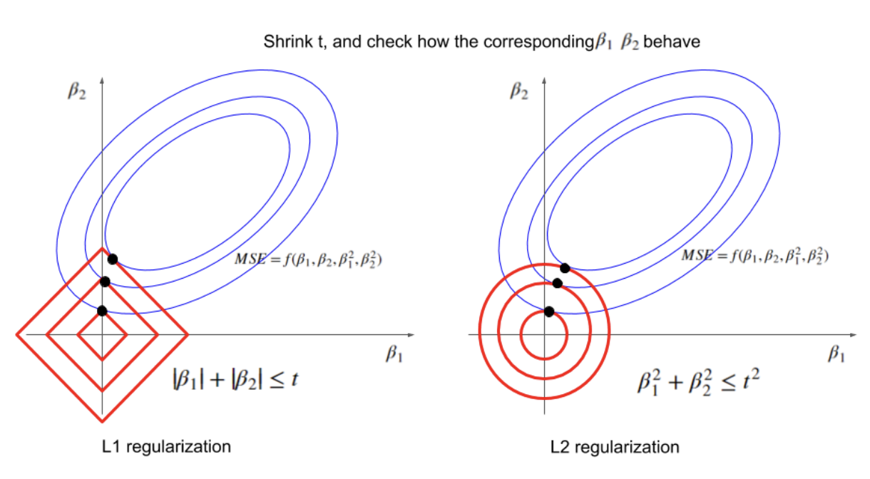 __Figure 3:__ Visualizing optimal values for parameters $ \beta_1 $ and $ \beta_2 $ under varying restrictions on $ t=r(\mathbf{\beta}) $. ([Xiaoli Chen, 2018](https://www.linkedin.com/pulse/intuitive-visual-explanation-differences-between-l1-l2-xiaoli-chen))
We consider an example where our goal is to minimize the mean squared error (MSE) loss subject to restrictions on parameters $ \beta_1 $ and $ \beta_2 $ imposed by $ L1 $ (left) and $ L2 $ (right) regularization.
Each red square / circle encloses all possible points such that $ \beta_1 $ and $ \beta_2 $ satisfy the $ L1 $ / $ L2 $ regularization condition for a fixed value of $ t $. The $ \beta_1, \beta_2 $ that minimize the MSE are those values at the point where the smallest possible ellipse (blue, representing the MSE) is tangent to the border of possible $ \beta_1, \beta_2 $ values (red). As $ t $ decreases, the optimal values of $ \beta_1 $ and $ \beta_2 $ get smaller for both $ L1 $ and $ L2 $ regularization, as expected; but the optimal values for $ \beta_1 $ and $ \beta_2 $ in $ L1 $ regularization are more likely to fall along an axis, near the "point" of the square (effectively zeroing out one parameter and encouraging sparsity). The [source](https://www.linkedin.com/pulse/intuitive-visual-explanation-differences-between-l1-l2-xiaoli-chen) for this example & explanation, also linked below the image, has a more in-depth exploration of this phenomenon.
## Regularization and Optimizers
Below we summarize the optimization problem and corresponding gradient update step for Empirical Risk Minimization with and without regularization, where $ \mathcal{D} $ is our dataset:
| Name | Optimization Problem | Gradient Update |
| :---: | :---: | :---: |
| ERM | $$\operatorname{argmin}_{\mathbf{w}} \mathcal{L}(\mathbf{w},\mathcal{D})$$ | $ \mathbf{w}_{t+1}=\mathbf{w}_t-\alpha\nabla\mathcal{L}(\mathbf{w}_t,\mathcal{D}) $ |
| ERM + $ L1 $ Reg. | $$\operatorname{argmin}_{\mathbf{w}} \mathcal{L}(\mathbf{w},\mathcal{D}) + \lambda \|\| \mathbf{w} \|\|_1 $$ | $$\mathbf{w}_{t+1}=\mathbf{w}_t-\alpha \nabla \mathcal{L}(\mathbf{w}_t,\mathcal{D})-\alpha\lambda \cdot \text{sgn}(\mathbf{w}_t)$$ |
| ERM + $ L2 $ Reg. | $$ \operatorname{argmin}_{\mathbf{w}} \mathcal{L}(\mathbf{w},\mathcal{D}) + \frac{\lambda}{2} \|\|\mathbf{w}\|\|_2^2 $$ | $$\mathbf{w}_{t+1}=\mathbf{w}_t-\alpha \nabla \mathcal{L}(\mathbf{w}_t,\mathcal{D})-\alpha\lambda \cdot \mathbf{w}_t$$
### Adam with L2 Regularization vs. Adam with Weight Decay (AdamW)
With traditional $ L2 $ regularization, the optimizer treats the regularizer just like loss. Hence, the gradient of the loss with respect to $ \mathbf{w}_t $ includes a term ($ \lambda \cdot \mathbf{w}_t $) from the regularizer, which we can see from our gradient update step:
$$ \mathbf{w}_{t+1}=\mathbf{w}_t-\alpha( \nabla \mathcal{L}(\mathbf{w}_t,\mathcal{D})+\lambda \cdot \mathbf{w}_t) $$
If we follow this same line of thinking—incorporating the regularization term into the loss, thus impacting the gradient of the loss function—for adaptive optimizers like Adam, we face an unintended consequence: we end up applying different regularization strengths to different parameters. Decoupling the regularization term from the gradient update (and instead incorporating it directly into the $ \mathbf{w}_t $ update) is the motivation behind AdamW.
#### Adam with L2 Regularization
Let's take a closer look. From above, the gradient at time $ t $ when using $ L2 $ regularization is given by
$$ \mathbf{g}_{t} = \nabla \mathcal{L}(\mathbf{w}_{t-1},\mathcal{D}) \ + \ \lambda \cdot \mathbf{w}_{t-1} $$
In traditional gradient descent, this regularization term is incorporated directly into the weight update $ \mathbf{w}_{t} $ (see above). But with *Adam*, an adaptive optimizer, we scale the learning rate for each parameter based on past gradients, which requires several additional computations before we ever update weights. Before computing $ \mathbf{w}_{t} $, we use $ \mathbf{g}_t $ to compute
$$\mathbf{m}_{t} = \beta_1\mathbf{m}_{t-1} + (1-\beta_1)\mathbf{g}_t \ \text{ and then } \ \mathbf{\hat{m}}_{t}=\frac{\mathbf{m}_{t}}{1-\beta_1^{t}}$$
$$ \mathbf{v}_{t} = \beta_2\mathbf{v}_{t-1}+(1-\beta_2)\mathbf{g}_t^2 \text{ and then } \mathbf{\hat{v}}_{t} = \frac{\mathbf{v}_{t}}{1-\beta_2^{t}} $$
which finally give us the weight update
$$ \mathbf{w}_{t} = \mathbf{w}_{t-1} - \frac{\alpha}{\sqrt{\mathbf{\hat{v}}_{t}+ \epsilon}} \odot \hat{\mathbf{m}}_{t}$$
The regularization term in $ \mathbf{g}_t $ gets "absorbed" into the $ \hat{\mathbf{v}}_t $ and $ \hat{\mathbf{m}}_t $ and then scaled by Adam's per-parameter learning rates. In other words, thanks to Adam's adaptive scaling, the effect of the regularization depends on the parameter's gradient history and momentum. This means parameters with small gradients may get almost no regularization, while others may get too much. We are essentially combining "how fast we learn" with "how much we regularize," which is not consistent with the goal of $ L2 $ regularization.
#### Adam with Weight Decay (AdamW)
AdamW behaves the way we *want* Adam with $ L2 $ regularization to behave, decoupling the weight decay from the gradient update and applying regularization more consistently across parameters. AdamW computes the gradient as
$$ \mathbf{g}_{t} = \nabla \mathcal{L}(\mathbf{w}_{t-1},\mathcal{D}) $$
(i.e., without the $ \lambda \cdot \mathbf{w}_{t-1} $ term from $ L2 $ regularization). We incorporate the regularization later, at weight update time:
$$ \mathbf{w}_t = \mathbf{w}_{t-1} - \ \eta_t \left(\frac{\alpha}{\sqrt{\hat{\mathbf{v}}_t + \epsilon}} \odot \hat{\mathbf{m}}_{t} + \lambda \cdot \mathbf{w}_{t-1} \right)$$
where $ \eta_t $ can be fixed or *decay* over time. Here, the magnitude of the term $ \lambda \cdot \mathbf{w}_{t-1} $ is no longer controlled by the particular learning rate $ \alpha $ for a given parameter. In practice, Adam with weight decay (AdamW) is more effective than using Adam with $ L2 $ regularization.
## Data Augmentation
Data augmentation is a regularization technique applied to the training data, rather than the model itself. To improve a model's robustness and decrease its sensitivity to noisy variations in the training data, we can diversify the training set with *label-preserving* transformations to the input data.
### Data Augmentation for Images
Data augmentation can be most easily visualized with image data. Changes in brightness, horizontal/vertical translations (like below), reflections, rotations, etc. are all transformations that *can* ultimately preserve the label of the data.
__Figure 3:__ Visualizing optimal values for parameters $ \beta_1 $ and $ \beta_2 $ under varying restrictions on $ t=r(\mathbf{\beta}) $. ([Xiaoli Chen, 2018](https://www.linkedin.com/pulse/intuitive-visual-explanation-differences-between-l1-l2-xiaoli-chen))
We consider an example where our goal is to minimize the mean squared error (MSE) loss subject to restrictions on parameters $ \beta_1 $ and $ \beta_2 $ imposed by $ L1 $ (left) and $ L2 $ (right) regularization.
Each red square / circle encloses all possible points such that $ \beta_1 $ and $ \beta_2 $ satisfy the $ L1 $ / $ L2 $ regularization condition for a fixed value of $ t $. The $ \beta_1, \beta_2 $ that minimize the MSE are those values at the point where the smallest possible ellipse (blue, representing the MSE) is tangent to the border of possible $ \beta_1, \beta_2 $ values (red). As $ t $ decreases, the optimal values of $ \beta_1 $ and $ \beta_2 $ get smaller for both $ L1 $ and $ L2 $ regularization, as expected; but the optimal values for $ \beta_1 $ and $ \beta_2 $ in $ L1 $ regularization are more likely to fall along an axis, near the "point" of the square (effectively zeroing out one parameter and encouraging sparsity). The [source](https://www.linkedin.com/pulse/intuitive-visual-explanation-differences-between-l1-l2-xiaoli-chen) for this example & explanation, also linked below the image, has a more in-depth exploration of this phenomenon.
## Regularization and Optimizers
Below we summarize the optimization problem and corresponding gradient update step for Empirical Risk Minimization with and without regularization, where $ \mathcal{D} $ is our dataset:
| Name | Optimization Problem | Gradient Update |
| :---: | :---: | :---: |
| ERM | $$\operatorname{argmin}_{\mathbf{w}} \mathcal{L}(\mathbf{w},\mathcal{D})$$ | $ \mathbf{w}_{t+1}=\mathbf{w}_t-\alpha\nabla\mathcal{L}(\mathbf{w}_t,\mathcal{D}) $ |
| ERM + $ L1 $ Reg. | $$\operatorname{argmin}_{\mathbf{w}} \mathcal{L}(\mathbf{w},\mathcal{D}) + \lambda \|\| \mathbf{w} \|\|_1 $$ | $$\mathbf{w}_{t+1}=\mathbf{w}_t-\alpha \nabla \mathcal{L}(\mathbf{w}_t,\mathcal{D})-\alpha\lambda \cdot \text{sgn}(\mathbf{w}_t)$$ |
| ERM + $ L2 $ Reg. | $$ \operatorname{argmin}_{\mathbf{w}} \mathcal{L}(\mathbf{w},\mathcal{D}) + \frac{\lambda}{2} \|\|\mathbf{w}\|\|_2^2 $$ | $$\mathbf{w}_{t+1}=\mathbf{w}_t-\alpha \nabla \mathcal{L}(\mathbf{w}_t,\mathcal{D})-\alpha\lambda \cdot \mathbf{w}_t$$
### Adam with L2 Regularization vs. Adam with Weight Decay (AdamW)
With traditional $ L2 $ regularization, the optimizer treats the regularizer just like loss. Hence, the gradient of the loss with respect to $ \mathbf{w}_t $ includes a term ($ \lambda \cdot \mathbf{w}_t $) from the regularizer, which we can see from our gradient update step:
$$ \mathbf{w}_{t+1}=\mathbf{w}_t-\alpha( \nabla \mathcal{L}(\mathbf{w}_t,\mathcal{D})+\lambda \cdot \mathbf{w}_t) $$
If we follow this same line of thinking—incorporating the regularization term into the loss, thus impacting the gradient of the loss function—for adaptive optimizers like Adam, we face an unintended consequence: we end up applying different regularization strengths to different parameters. Decoupling the regularization term from the gradient update (and instead incorporating it directly into the $ \mathbf{w}_t $ update) is the motivation behind AdamW.
#### Adam with L2 Regularization
Let's take a closer look. From above, the gradient at time $ t $ when using $ L2 $ regularization is given by
$$ \mathbf{g}_{t} = \nabla \mathcal{L}(\mathbf{w}_{t-1},\mathcal{D}) \ + \ \lambda \cdot \mathbf{w}_{t-1} $$
In traditional gradient descent, this regularization term is incorporated directly into the weight update $ \mathbf{w}_{t} $ (see above). But with *Adam*, an adaptive optimizer, we scale the learning rate for each parameter based on past gradients, which requires several additional computations before we ever update weights. Before computing $ \mathbf{w}_{t} $, we use $ \mathbf{g}_t $ to compute
$$\mathbf{m}_{t} = \beta_1\mathbf{m}_{t-1} + (1-\beta_1)\mathbf{g}_t \ \text{ and then } \ \mathbf{\hat{m}}_{t}=\frac{\mathbf{m}_{t}}{1-\beta_1^{t}}$$
$$ \mathbf{v}_{t} = \beta_2\mathbf{v}_{t-1}+(1-\beta_2)\mathbf{g}_t^2 \text{ and then } \mathbf{\hat{v}}_{t} = \frac{\mathbf{v}_{t}}{1-\beta_2^{t}} $$
which finally give us the weight update
$$ \mathbf{w}_{t} = \mathbf{w}_{t-1} - \frac{\alpha}{\sqrt{\mathbf{\hat{v}}_{t}+ \epsilon}} \odot \hat{\mathbf{m}}_{t}$$
The regularization term in $ \mathbf{g}_t $ gets "absorbed" into the $ \hat{\mathbf{v}}_t $ and $ \hat{\mathbf{m}}_t $ and then scaled by Adam's per-parameter learning rates. In other words, thanks to Adam's adaptive scaling, the effect of the regularization depends on the parameter's gradient history and momentum. This means parameters with small gradients may get almost no regularization, while others may get too much. We are essentially combining "how fast we learn" with "how much we regularize," which is not consistent with the goal of $ L2 $ regularization.
#### Adam with Weight Decay (AdamW)
AdamW behaves the way we *want* Adam with $ L2 $ regularization to behave, decoupling the weight decay from the gradient update and applying regularization more consistently across parameters. AdamW computes the gradient as
$$ \mathbf{g}_{t} = \nabla \mathcal{L}(\mathbf{w}_{t-1},\mathcal{D}) $$
(i.e., without the $ \lambda \cdot \mathbf{w}_{t-1} $ term from $ L2 $ regularization). We incorporate the regularization later, at weight update time:
$$ \mathbf{w}_t = \mathbf{w}_{t-1} - \ \eta_t \left(\frac{\alpha}{\sqrt{\hat{\mathbf{v}}_t + \epsilon}} \odot \hat{\mathbf{m}}_{t} + \lambda \cdot \mathbf{w}_{t-1} \right)$$
where $ \eta_t $ can be fixed or *decay* over time. Here, the magnitude of the term $ \lambda \cdot \mathbf{w}_{t-1} $ is no longer controlled by the particular learning rate $ \alpha $ for a given parameter. In practice, Adam with weight decay (AdamW) is more effective than using Adam with $ L2 $ regularization.
## Data Augmentation
Data augmentation is a regularization technique applied to the training data, rather than the model itself. To improve a model's robustness and decrease its sensitivity to noisy variations in the training data, we can diversify the training set with *label-preserving* transformations to the input data.
### Data Augmentation for Images
Data augmentation can be most easily visualized with image data. Changes in brightness, horizontal/vertical translations (like below), reflections, rotations, etc. are all transformations that *can* ultimately preserve the label of the data.
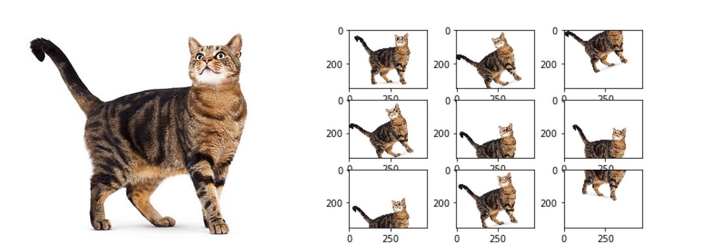 **Figure 4:** Examples of data augmentation on a photo of a cat ([Medium, 2024](https://medium.com/@saiwadotai/the-essential-guide-to-data-augmentation-in-deep-learning-f66e0907cdc8))
> *Note:* The kinds of transformations that preserve label depend greatly on the nature of the input. For example, rotating the digit “6” by 180° in a digit-recognition task does **not** preserve label, as the transformed image would belong to the “9” class.
### Data Augmentation for Text
Text augmentation can be a far more daunting task. Consider the task of classifying movie reviews as good or bad. Given a good review, it is difficult to think of many transformations that will preserve the "good" label. One possibility is to replace a few words with synonyms, but it is far less intuitive than transforming image data.
## DropOut
Dropout is a regularization technique that comes into play during both training and inference for a given model. Dropout works by randomly setting certain neurons to $ 0 $ (effectively "dropping" them) during each forward pass. The probability of keeping any given neuron, $ p $, is a hyperparameter. Commonly, we set $ p = 0.5 $.
**Figure 4:** Examples of data augmentation on a photo of a cat ([Medium, 2024](https://medium.com/@saiwadotai/the-essential-guide-to-data-augmentation-in-deep-learning-f66e0907cdc8))
> *Note:* The kinds of transformations that preserve label depend greatly on the nature of the input. For example, rotating the digit “6” by 180° in a digit-recognition task does **not** preserve label, as the transformed image would belong to the “9” class.
### Data Augmentation for Text
Text augmentation can be a far more daunting task. Consider the task of classifying movie reviews as good or bad. Given a good review, it is difficult to think of many transformations that will preserve the "good" label. One possibility is to replace a few words with synonyms, but it is far less intuitive than transforming image data.
## DropOut
Dropout is a regularization technique that comes into play during both training and inference for a given model. Dropout works by randomly setting certain neurons to $ 0 $ (effectively "dropping" them) during each forward pass. The probability of keeping any given neuron, $ p $, is a hyperparameter. Commonly, we set $ p = 0.5 $.
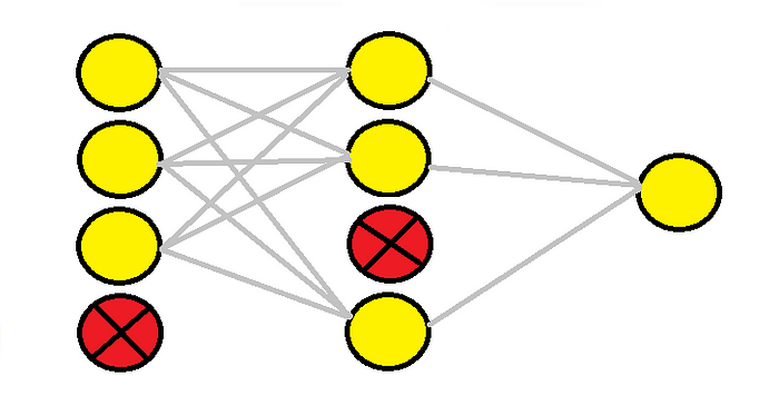 **Figure 5:** Two Dropout layers ([Comet, 2022](https://www.comet.com/site/blog/dropout-regularization-with-tensorflow-keras/))
### Why is DropOut a good idea?
* Forces a network to have redundant representations.
This prevents the network from relying too heavily on any single feature and reduces co-adaptation. Intuitively, this means that multiple features will end up being "required" to support correct classifications, causing a model to better generalize to noisy, unseen data.
* Creates an enormous *ensemble* of deep networks.
From our studies of *ensemble methods*, especially their usage in the realm of decision tree models, we know that averaging results across a collection of models acts as a regularizer. With dropout, we can think of each dropout mask as forming a "new" network.
For a fully connected layer with $ 4096 $ units, there are $ 2^{4096} \approx 10^{1233} $ possible dropout masks. Contrast that with the ~$ 10^{82} $ atoms in the universe!
### Implementing DropOut
#### Training
Implementing dropout at training time involves randomly dropping each neuron (i.e., setting it to $ 0 $) with probability $ 1-p $ during a forward pass, where $ p $ is the probability of keeping a neuron. If a neuron is dropped, the gradients of its associated weights are zero, so those weights are not updated during that training step.
#### Test Time
During test time, all neurons are used (none are dropped). However, to account for the training-time dropout, we scale each neuron by $ p $ at inference time.
Concretely: suppose a given neuron has activation $ a \in \mathbb{R} $. During training (with dropout), the expected value of $ a $ is $ \mathbb{E}[a]=p\cdot a $. During test time, though, the expected value of $ a $ would still be $ \mathbb{E}[a]=a $ since we use all nodes.
To fix this mismatch in expectation, we simply scale the activations by a factor of $ p $ at test time so that $ \mathbb{E}[a]=p\cdot a $ more closely resembles (in expectation) the network we had during training.
> *Some class conventions:* Other sources commonly use $ p $ to represent the probability of *dropping* any given neuron. In CS4782 we use $ p $ as the probability of *keeping* any given neuron. Additionally, many sources also apply rescaling during training time by scaling training activations by $ 1/p $. While these two methods are equivalent in expectation, the general CS4782 convention applies rescaling at *test* time.
## BatchNorm
Batch normalization is not a traditional regularizer itself, but rather a technique that leads to regularizer-like behavior in model performance.
Consider a deep learning task that aims to predict house prices. Let $ x_1 $ be a feature representing bedroom number $ \in [1,5] $ and let $ x_2 $ be a feature representing square footage $ \in [0, 2000] $. Common sense tells us that a change in the number of bedrooms by $ 1 $ bedroom should have a substantial impact on home price, whereas a $ 1\text{ft}^2 $ increase will have a far smaller impact on the home price. In deep networks, however, we typically do not know *a priori* which features will be significantly relevant, and thus the contour map of the loss function in this example may look like the figure on the left:
**Figure 5:** Two Dropout layers ([Comet, 2022](https://www.comet.com/site/blog/dropout-regularization-with-tensorflow-keras/))
### Why is DropOut a good idea?
* Forces a network to have redundant representations.
This prevents the network from relying too heavily on any single feature and reduces co-adaptation. Intuitively, this means that multiple features will end up being "required" to support correct classifications, causing a model to better generalize to noisy, unseen data.
* Creates an enormous *ensemble* of deep networks.
From our studies of *ensemble methods*, especially their usage in the realm of decision tree models, we know that averaging results across a collection of models acts as a regularizer. With dropout, we can think of each dropout mask as forming a "new" network.
For a fully connected layer with $ 4096 $ units, there are $ 2^{4096} \approx 10^{1233} $ possible dropout masks. Contrast that with the ~$ 10^{82} $ atoms in the universe!
### Implementing DropOut
#### Training
Implementing dropout at training time involves randomly dropping each neuron (i.e., setting it to $ 0 $) with probability $ 1-p $ during a forward pass, where $ p $ is the probability of keeping a neuron. If a neuron is dropped, the gradients of its associated weights are zero, so those weights are not updated during that training step.
#### Test Time
During test time, all neurons are used (none are dropped). However, to account for the training-time dropout, we scale each neuron by $ p $ at inference time.
Concretely: suppose a given neuron has activation $ a \in \mathbb{R} $. During training (with dropout), the expected value of $ a $ is $ \mathbb{E}[a]=p\cdot a $. During test time, though, the expected value of $ a $ would still be $ \mathbb{E}[a]=a $ since we use all nodes.
To fix this mismatch in expectation, we simply scale the activations by a factor of $ p $ at test time so that $ \mathbb{E}[a]=p\cdot a $ more closely resembles (in expectation) the network we had during training.
> *Some class conventions:* Other sources commonly use $ p $ to represent the probability of *dropping* any given neuron. In CS4782 we use $ p $ as the probability of *keeping* any given neuron. Additionally, many sources also apply rescaling during training time by scaling training activations by $ 1/p $. While these two methods are equivalent in expectation, the general CS4782 convention applies rescaling at *test* time.
## BatchNorm
Batch normalization is not a traditional regularizer itself, but rather a technique that leads to regularizer-like behavior in model performance.
Consider a deep learning task that aims to predict house prices. Let $ x_1 $ be a feature representing bedroom number $ \in [1,5] $ and let $ x_2 $ be a feature representing square footage $ \in [0, 2000] $. Common sense tells us that a change in the number of bedrooms by $ 1 $ bedroom should have a substantial impact on home price, whereas a $ 1\text{ft}^2 $ increase will have a far smaller impact on the home price. In deep networks, however, we typically do not know *a priori* which features will be significantly relevant, and thus the contour map of the loss function in this example may look like the figure on the left:
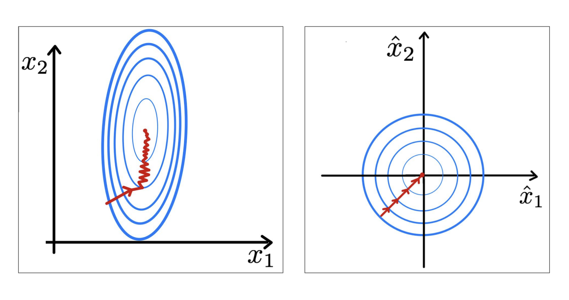 **Figure 6:** Unnormalized (left) and normalized (right) features with loss contour ([LeCun et al., 1998](http://vision.stanford.edu/cs598_spring07/papers/Lecun98.pdf))
If we instead normalize the features across a batch of training points $ \mathcal{B}=\{\mathbf{x_1},...,\mathbf{x_m}\} $:
$$\hat{\mathbf{x}}_i \leftarrow \frac{\mathbf{x}_i - \mathbf{\mu}_{\mathcal{B}}}{\sqrt{\mathbf{\sigma}_{\mathcal{B}}^2 + \epsilon}}$$
where $ \epsilon $ is a small, positive constant (mainly there to prevent division-by-zero) and $ \mathbf{\mu}_{\mathcal{B}} $ and $ \mathbf{\sigma}_{\mathcal{B}} $ are the mean and standard deviation of all $ \mathbf{x}_i \in \mathcal{B} $, respectively, we see that the contour map of the loss function becomes far more balanced, or spherical, like the plot on the right.
In short, batch normalization ensures features have a similar scale (unlike the bedroom number vs. square footage scenario) by standardizing each feature and then optimally rescaling and shifting using learnable parameters $ \gamma $ and $ \beta $.
### Why Does This Matter?
Using our knowledge of optimization methods like gradient descent, we know that optimizers take steps *perpendicular* to the contour lines of the loss function. In the figure on the left, we see that we must take very small steps (small learning rate) to avoid overshooting one feature (bedroom number) and then are forced to take small steps through the deep valleys trying to find the sweet spot on $ x_2 $.
In the case of standardized features, our loss function is far smoother, and we can thus use a larger learning rate to find the minima more quickly.
One chief advantage of this is quite apparent: using a larger learning rate speeds up the optimization process greatly, a benefit during training. We will discuss another effect later that has a regularizing effect on model performance.
### Batch Normalization in Deep Networks
In deep networks, batch normalization appears as another layer in between two hidden layers. The batch normalization layer normalizes the activations output from one layer before passing them as inputs to the next hidden layer. In PyTorch, we use `torch.nn.BatchNorm1d` for 2D or 3D inputs.
#### The Batch Normalization Algorithm
The following algorithm applies the *Batch Normalization Transform* to activation $ \mathbf{x}_i $ over a mini-batch.
**Input:** Values of $ \mathbf{x}_i $ over a mini-batch: $ \mathcal{B} = \{\mathbf{x}_1...\mathbf{x}_m\} $;
Parameters to be learned: $ \gamma, \beta $
**Output:** $ \{y_i = \text{BN}_{\gamma,\beta}(\mathbf{x}_i)\} $
$$\mu_\mathcal{B} \leftarrow \frac{1}{m}\sum_{i=1}^{m} \mathbf{x}_i \qquad \text{// mini-batch mean}$$
$$\sigma_\mathcal{B}^2 \leftarrow \frac{1}{m}\sum_{i=1}^{m} (\mathbf{x}_i - \mu_\mathcal{B})^2 \qquad \text{// mini-batch variance}$$
$$\hat{\mathbf{x}}_i \leftarrow \frac{\mathbf{x}_i - \mu_\mathcal{B}}{\sqrt{\sigma_\mathcal{B}^2 + \epsilon}} \qquad \text{// normalize}$$
$$\mathbf{y}_i \leftarrow \gamma\hat{\mathbf{x}}_i + \beta \equiv \text{BN}_{\gamma,\beta}(\mathbf{x}_i) \qquad \text{// scale and shift}$$
#### Inference Behavior
At inference time, taking the mean and variance of one sample, or batch, gives us a very noisy and unreliable estimate of population statistics. This can cause a model to be nondeterministic, or provide different outputs given the same inputs. To abate this issue, we instead use (at inference time) running average statistics calculated during training as
$$\mu_{inf} = \lambda\mu_{inf} + (1 - \lambda)\mu_{\mathcal{B}}$$
$$\sigma_{inf}^2 = \lambda\sigma_{inf}^2 + (1 - \lambda)\sigma_{\mathcal{B}}^2$$
where $ \lambda $ is a momentum parameter (a constant, usually ~$ 0.9 $), and $ \mu_{\mathcal{B}} $ and $ \sigma_{\mathcal{B}}^2 $ are the mean and variance, respectively, of a mini-batch during training.
These running average statistics serve as good estimates of population mean and variance and give us deterministic behavior during inference time.
### Benefits of Batch Normalization
We have already discussed how batch normalization allows us to use a larger learning rate and thus speeds up optimization. Another advantage of using a larger learning rate is that a network may *generalize* better: the core aim of regularization.
**Figure 6:** Unnormalized (left) and normalized (right) features with loss contour ([LeCun et al., 1998](http://vision.stanford.edu/cs598_spring07/papers/Lecun98.pdf))
If we instead normalize the features across a batch of training points $ \mathcal{B}=\{\mathbf{x_1},...,\mathbf{x_m}\} $:
$$\hat{\mathbf{x}}_i \leftarrow \frac{\mathbf{x}_i - \mathbf{\mu}_{\mathcal{B}}}{\sqrt{\mathbf{\sigma}_{\mathcal{B}}^2 + \epsilon}}$$
where $ \epsilon $ is a small, positive constant (mainly there to prevent division-by-zero) and $ \mathbf{\mu}_{\mathcal{B}} $ and $ \mathbf{\sigma}_{\mathcal{B}} $ are the mean and standard deviation of all $ \mathbf{x}_i \in \mathcal{B} $, respectively, we see that the contour map of the loss function becomes far more balanced, or spherical, like the plot on the right.
In short, batch normalization ensures features have a similar scale (unlike the bedroom number vs. square footage scenario) by standardizing each feature and then optimally rescaling and shifting using learnable parameters $ \gamma $ and $ \beta $.
### Why Does This Matter?
Using our knowledge of optimization methods like gradient descent, we know that optimizers take steps *perpendicular* to the contour lines of the loss function. In the figure on the left, we see that we must take very small steps (small learning rate) to avoid overshooting one feature (bedroom number) and then are forced to take small steps through the deep valleys trying to find the sweet spot on $ x_2 $.
In the case of standardized features, our loss function is far smoother, and we can thus use a larger learning rate to find the minima more quickly.
One chief advantage of this is quite apparent: using a larger learning rate speeds up the optimization process greatly, a benefit during training. We will discuss another effect later that has a regularizing effect on model performance.
### Batch Normalization in Deep Networks
In deep networks, batch normalization appears as another layer in between two hidden layers. The batch normalization layer normalizes the activations output from one layer before passing them as inputs to the next hidden layer. In PyTorch, we use `torch.nn.BatchNorm1d` for 2D or 3D inputs.
#### The Batch Normalization Algorithm
The following algorithm applies the *Batch Normalization Transform* to activation $ \mathbf{x}_i $ over a mini-batch.
**Input:** Values of $ \mathbf{x}_i $ over a mini-batch: $ \mathcal{B} = \{\mathbf{x}_1...\mathbf{x}_m\} $;
Parameters to be learned: $ \gamma, \beta $
**Output:** $ \{y_i = \text{BN}_{\gamma,\beta}(\mathbf{x}_i)\} $
$$\mu_\mathcal{B} \leftarrow \frac{1}{m}\sum_{i=1}^{m} \mathbf{x}_i \qquad \text{// mini-batch mean}$$
$$\sigma_\mathcal{B}^2 \leftarrow \frac{1}{m}\sum_{i=1}^{m} (\mathbf{x}_i - \mu_\mathcal{B})^2 \qquad \text{// mini-batch variance}$$
$$\hat{\mathbf{x}}_i \leftarrow \frac{\mathbf{x}_i - \mu_\mathcal{B}}{\sqrt{\sigma_\mathcal{B}^2 + \epsilon}} \qquad \text{// normalize}$$
$$\mathbf{y}_i \leftarrow \gamma\hat{\mathbf{x}}_i + \beta \equiv \text{BN}_{\gamma,\beta}(\mathbf{x}_i) \qquad \text{// scale and shift}$$
#### Inference Behavior
At inference time, taking the mean and variance of one sample, or batch, gives us a very noisy and unreliable estimate of population statistics. This can cause a model to be nondeterministic, or provide different outputs given the same inputs. To abate this issue, we instead use (at inference time) running average statistics calculated during training as
$$\mu_{inf} = \lambda\mu_{inf} + (1 - \lambda)\mu_{\mathcal{B}}$$
$$\sigma_{inf}^2 = \lambda\sigma_{inf}^2 + (1 - \lambda)\sigma_{\mathcal{B}}^2$$
where $ \lambda $ is a momentum parameter (a constant, usually ~$ 0.9 $), and $ \mu_{\mathcal{B}} $ and $ \sigma_{\mathcal{B}}^2 $ are the mean and variance, respectively, of a mini-batch during training.
These running average statistics serve as good estimates of population mean and variance and give us deterministic behavior during inference time.
### Benefits of Batch Normalization
We have already discussed how batch normalization allows us to use a larger learning rate and thus speeds up optimization. Another advantage of using a larger learning rate is that a network may *generalize* better: the core aim of regularization.
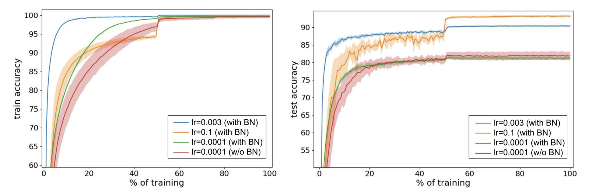 **Figure 7:** ([Bjorck et al., 2018](https://arxiv.org/abs/1806.02375))
The above figure illustrates the regularizing characteristics that appear when BatchNorm is applied in conjunction with a larger learning rate. At small learning rates (green vs. red), the inclusion of BatchNorm layers does not have an impact on test accuracy (right). When we increase the learning rates (blue, orange), however, we see that test accuracy improves drastically by reducing overfitting and generalizing better to unseen data. This improvement is a direct effect of the larger learning rate that we were able to use by including BatchNorm layers in the network.
### Why Does a Larger Learning Rate Generalize Better?
During optimization, the noise of the gradient estimate scales with the learning rate. Noisy gradient estimates during optimization are the core of Stochastic Gradient Descent (SGD) as well, which we know improves upon traditional Gradient Descent due to SGD's capacity to escape local minima and find smoother, more general solutions.
Therefore, the noisy gradient estimates from using a larger learning rate help find more global, generalizable solutions in the same manner as SGD.
> *Note:* This behavior is not exclusive to large learning rate optimization. By adding Gaussian noise to the activations of a network during training time we can still see this regularizing effect even at smaller learning rates:
**Figure 7:** ([Bjorck et al., 2018](https://arxiv.org/abs/1806.02375))
The above figure illustrates the regularizing characteristics that appear when BatchNorm is applied in conjunction with a larger learning rate. At small learning rates (green vs. red), the inclusion of BatchNorm layers does not have an impact on test accuracy (right). When we increase the learning rates (blue, orange), however, we see that test accuracy improves drastically by reducing overfitting and generalizing better to unseen data. This improvement is a direct effect of the larger learning rate that we were able to use by including BatchNorm layers in the network.
### Why Does a Larger Learning Rate Generalize Better?
During optimization, the noise of the gradient estimate scales with the learning rate. Noisy gradient estimates during optimization are the core of Stochastic Gradient Descent (SGD) as well, which we know improves upon traditional Gradient Descent due to SGD's capacity to escape local minima and find smoother, more general solutions.
Therefore, the noisy gradient estimates from using a larger learning rate help find more global, generalizable solutions in the same manner as SGD.
> *Note:* This behavior is not exclusive to large learning rate optimization. By adding Gaussian noise to the activations of a network during training time we can still see this regularizing effect even at smaller learning rates:
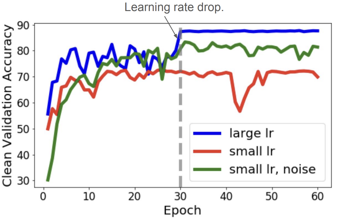 **Figure 8:** Validation accuracy when using a large learning rate, small learning rate, and a small learning rate + noise ([Li et. al., 2019](https://arxiv.org/abs/1907.04595))
## Deep Double Descent
Deep double descent is not a regularization technique, but rather a behavior exhibited by large, *regularized* models that may seem rather counterintuitive.
**Figure 8:** Validation accuracy when using a large learning rate, small learning rate, and a small learning rate + noise ([Li et. al., 2019](https://arxiv.org/abs/1907.04595))
## Deep Double Descent
Deep double descent is not a regularization technique, but rather a behavior exhibited by large, *regularized* models that may seem rather counterintuitive.
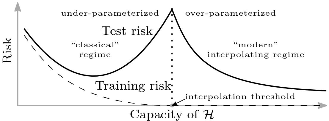 **Figure 9:** Empirical risk curve ([Belkin et. al, 2019](https://arxiv.org/abs/1812.11118))
Looking at the above empirical risk curve, we are familiar with the classic U-shaped curve to the left of the interpolation threshold. Far to the left, our model is clearly underfitting and we must increase the capacity of the model to improve accuracy. Move too far along the curve, however, and we see overfitting begin to occur where the model is "over-parameterized" and poorly generalizes to unseen data.
In traditional empirical risk minimization (ERM) with a regularizer, we know that the optimization problem is as follows, with $ r(h) $ being some measure of model complexity:
$$h = \operatorname{argmin}_{h \in \mathcal{H}} \mathcal{L}(h) + \lambda \cdot r(h)$$
At the interpolation threshold, $ \mathcal{L}(h) \approx 0 $ since the model fits the training data perfectly. Thus, ERM becomes
$$
h = \operatorname{argmin}_{h \in \mathcal{H}} \mathcal{L}(h) + \lambda \cdot r(h)
\approx
\operatorname{argmin}_{h \in \{h : \mathcal{L}(h) \approx 0\}} r(h)
$$
Past the interpolation threshold, there are an infinite number of solutions that perfectly fit the data. Therefore, the new minimization problem in the interpolating regime is equivalent to just minimizing the regularizer, i.e., finding the simplest solution that perfectly fits the data.
By finding simpler solutions, we anticipate that the model will generalize better, and empirical evidence shows this to be the case in complex modern architectures like ResNet and Transformers!
**Figure 9:** Empirical risk curve ([Belkin et. al, 2019](https://arxiv.org/abs/1812.11118))
Looking at the above empirical risk curve, we are familiar with the classic U-shaped curve to the left of the interpolation threshold. Far to the left, our model is clearly underfitting and we must increase the capacity of the model to improve accuracy. Move too far along the curve, however, and we see overfitting begin to occur where the model is "over-parameterized" and poorly generalizes to unseen data.
In traditional empirical risk minimization (ERM) with a regularizer, we know that the optimization problem is as follows, with $ r(h) $ being some measure of model complexity:
$$h = \operatorname{argmin}_{h \in \mathcal{H}} \mathcal{L}(h) + \lambda \cdot r(h)$$
At the interpolation threshold, $ \mathcal{L}(h) \approx 0 $ since the model fits the training data perfectly. Thus, ERM becomes
$$
h = \operatorname{argmin}_{h \in \mathcal{H}} \mathcal{L}(h) + \lambda \cdot r(h)
\approx
\operatorname{argmin}_{h \in \{h : \mathcal{L}(h) \approx 0\}} r(h)
$$
Past the interpolation threshold, there are an infinite number of solutions that perfectly fit the data. Therefore, the new minimization problem in the interpolating regime is equivalent to just minimizing the regularizer, i.e., finding the simplest solution that perfectly fits the data.
By finding simpler solutions, we anticipate that the model will generalize better, and empirical evidence shows this to be the case in complex modern architectures like ResNet and Transformers!