# Modern ConvNets
## Recap: Deeper CNN Architecture
Recall from the previous lecture that stacking two $ 3 \times 3 $ convolutional layers can outperform a single $ 5 \times 5 $ convolutional layer:
 In general, deeper architectures allow models to learn more complex and hierarchical features: early layers detect simple patterns like edges and textures, while later layers combine these into structures like shapes and objects. Stacking many layers together lets the network learn more expressive functions and achieve better performance.
However, increasing depth also introduces significant optimization challenges.
### Challenges with Deeper Architectures
In the graph below, the deeper, $ 56 $-layer CNN has a higher training *and* test error than the shallower, $ 20 $-layer CNN. This implies that the deeper network is underfitting—but why?
In general, deeper architectures allow models to learn more complex and hierarchical features: early layers detect simple patterns like edges and textures, while later layers combine these into structures like shapes and objects. Stacking many layers together lets the network learn more expressive functions and achieve better performance.
However, increasing depth also introduces significant optimization challenges.
### Challenges with Deeper Architectures
In the graph below, the deeper, $ 56 $-layer CNN has a higher training *and* test error than the shallower, $ 20 $-layer CNN. This implies that the deeper network is underfitting—but why?
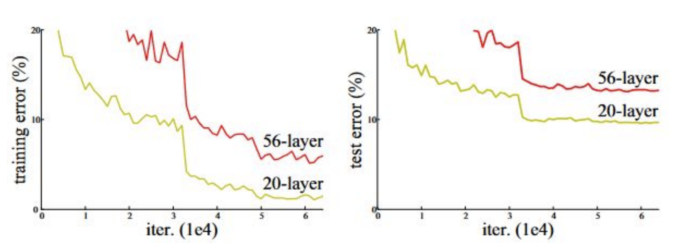 **Figure 1:** Train and test error of a $ 56 $-layer CNN (red) vs. a $ 20 $-layer CNN (green) on an image classification test with the CIFAR-10 dataset ([He et al., "Deep residual learning for image recognition," 2016](https://arxiv.org/abs/1512.03385))
There are two main problems with these deeper networks:
1. The **longer training** time required to train a network of that size, and
2. **Vanishing gradients**. The long, chained gradient calculations that come with backpropagating through these deeper models means that the gradients approach zero, which leads to unhelpful weight updates and halts learning.
Deeper and wider networks become more expensive in terms of compute power, memory, and run time; the more parameters a model has, the more operations it executes during a forward pass. This brings us to our goal: given a fixed computational budget, we want to optimize the depth and width of our network.
## GoogLeNet
Also called InceptionNet (after the [viral meme](https://lh3.googleusercontent.com/proxy/eFTG7D9NiWzU0LQNfINb0CRG3STrL1wfSveiVgQjoUZ_4NHkoCpQZV8tdD3Mlz_-kuZpS3f19YezjggcG4UaB6sJod4ZAfkf8vQhMby1iIKNC-mWbYGkAh39lA_3SSQuTr9Bu_fR5P_9uxBB35e0gNGsfKiR) from the movie *Inception*), GoogLeNet was one of the first deep CNN architectures. It is known for introducing the Inception Module as the main building block of the network and using $ 1 \times 1 $ convolutions to reduce computational cost.
### Inception Module [Version 1]
The Inception module is the main building block of GoogLeNet:
**Figure 1:** Train and test error of a $ 56 $-layer CNN (red) vs. a $ 20 $-layer CNN (green) on an image classification test with the CIFAR-10 dataset ([He et al., "Deep residual learning for image recognition," 2016](https://arxiv.org/abs/1512.03385))
There are two main problems with these deeper networks:
1. The **longer training** time required to train a network of that size, and
2. **Vanishing gradients**. The long, chained gradient calculations that come with backpropagating through these deeper models means that the gradients approach zero, which leads to unhelpful weight updates and halts learning.
Deeper and wider networks become more expensive in terms of compute power, memory, and run time; the more parameters a model has, the more operations it executes during a forward pass. This brings us to our goal: given a fixed computational budget, we want to optimize the depth and width of our network.
## GoogLeNet
Also called InceptionNet (after the [viral meme](https://lh3.googleusercontent.com/proxy/eFTG7D9NiWzU0LQNfINb0CRG3STrL1wfSveiVgQjoUZ_4NHkoCpQZV8tdD3Mlz_-kuZpS3f19YezjggcG4UaB6sJod4ZAfkf8vQhMby1iIKNC-mWbYGkAh39lA_3SSQuTr9Bu_fR5P_9uxBB35e0gNGsfKiR) from the movie *Inception*), GoogLeNet was one of the first deep CNN architectures. It is known for introducing the Inception Module as the main building block of the network and using $ 1 \times 1 $ convolutions to reduce computational cost.
### Inception Module [Version 1]
The Inception module is the main building block of GoogLeNet:
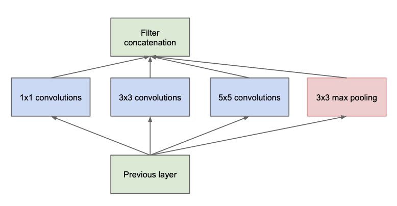 **Figure 2:** Diagram of an Inception Module (without dimension reduction) ([Szegedy et al., "Going deeper with convolutions," 2015](https://arxiv.org/abs/1409.4842))
In each Inception module, we have parallel $ 1\times 1 $, $ 3 \times 3 $, and $ 5 \times 5 $ convolution layers as well as a $ 3 \times 3 $ max pooling layer. As we will see, this is quite computationally expensive.
**Number of Parameters**
The number of parameters in a convolutional layer is $$H\times W\times C\times F$$ where $ H $ and $ W $ are the filter height and width, $ C $ is the number of input channels, and $ F $ is the number of filters.
With $ C $ input channels and $ F $ filters:
* The $ 3 \times 3 $ convolution has $ 3*3*C*F= 9CF $ parameters
- The $ 5 \times 5 $ convolution has $ 5*5*C*F = 25CF $ parameters
Notice that the number of parameters scales linearly with the number of input channels (and with the number of filters). When multiple Inception modules are chained together to create the full network, this adds up quickly.
**Number of Channels**
In an Inception module, the output channels of all branches (convolution and max pooling) are *concatenated* to form the module's final output
- Convolutional Layers: The number of output channels equals the number of filters, $ F $
- Max Pooling ($ 3\times 3 $): The number of output channels equals the number of input channels $ C $
Since the pooling output is concatenated with the convolution outputs, the total number of channels increases. This larger output becomes the *input* to the next Inception module. As a result, the number of channels (and thus the number of parameters in successive modules) accumulates rapidly.
To control this growth, GoogLeNet uses Inception modules with dimension reduction ($ 1\times 1 $ convolutions) to limit the number of output channels.
### $ 1\times 1 $ Convolutions
We can use $ 1\times 1 $ convolutions to change the number of channels while preserving the height and width of the input.

**Figure 3:** Using two $ 1 \times 1 $ convolutional filters to go from $ C=4 $ to $ C=2 $ channels.
As a more concrete example, the following shows sample calculations with $ 1 \times 1 $ convolutional filters:

**Figure 4:** Sample calculations for applying $ 1 \times 1 $ convolutional filters.
To reiterate, reducing the number of channels is key for reducing total parameter count because successive layers will need fewer (filter) parameters.
### Impact of Dimension Reduction
To further illustrate the importance of dimension reduction, we will consider two different architectures that have the same number of input and output channels but vastly different parameter counts due to intermediate dimension reduction.
Given an input with $ 256 $ channels:
1. **Architecture 1:** $ 3 \times 3 $ convolution with $ 256 $ filters
2. **Architecture 2:** $ 1 \times 1 $ convolution with $ 64 $ filters $ \to $ $ 3\times 3 $ convolution with $ 64 $ filters $ \to $ $ 1 \times 1 $ convolution with $ 256 $ filters
>Try it out yourself: how many parameters does each model have? *Recall: The number of parameters of a convolutional layer $ = H\times W\times C\times F $*
1. **Architecture 1:** $ 3*3*256*256 = 589,824 $ parameters
2. **Architecture 2:** $ 1*1*256*64 + 3*3*64*64 + 1*1*64*256 = 69,632 $ parameters
Using our $ 1 \times 1 $ filters before and after the $ 3 \times 3 $ filter to reduce intermediate channels allowed us to go from ~$ 590,000 $ to just ~$ 70,000 $ parameters.
### Inception Module [Version 2]
The final version of the Inception module includes these $ 1 \times 1 $ convolutions for channel and parameter reduction:
**Figure 2:** Diagram of an Inception Module (without dimension reduction) ([Szegedy et al., "Going deeper with convolutions," 2015](https://arxiv.org/abs/1409.4842))
In each Inception module, we have parallel $ 1\times 1 $, $ 3 \times 3 $, and $ 5 \times 5 $ convolution layers as well as a $ 3 \times 3 $ max pooling layer. As we will see, this is quite computationally expensive.
**Number of Parameters**
The number of parameters in a convolutional layer is $$H\times W\times C\times F$$ where $ H $ and $ W $ are the filter height and width, $ C $ is the number of input channels, and $ F $ is the number of filters.
With $ C $ input channels and $ F $ filters:
* The $ 3 \times 3 $ convolution has $ 3*3*C*F= 9CF $ parameters
- The $ 5 \times 5 $ convolution has $ 5*5*C*F = 25CF $ parameters
Notice that the number of parameters scales linearly with the number of input channels (and with the number of filters). When multiple Inception modules are chained together to create the full network, this adds up quickly.
**Number of Channels**
In an Inception module, the output channels of all branches (convolution and max pooling) are *concatenated* to form the module's final output
- Convolutional Layers: The number of output channels equals the number of filters, $ F $
- Max Pooling ($ 3\times 3 $): The number of output channels equals the number of input channels $ C $
Since the pooling output is concatenated with the convolution outputs, the total number of channels increases. This larger output becomes the *input* to the next Inception module. As a result, the number of channels (and thus the number of parameters in successive modules) accumulates rapidly.
To control this growth, GoogLeNet uses Inception modules with dimension reduction ($ 1\times 1 $ convolutions) to limit the number of output channels.
### $ 1\times 1 $ Convolutions
We can use $ 1\times 1 $ convolutions to change the number of channels while preserving the height and width of the input.

**Figure 3:** Using two $ 1 \times 1 $ convolutional filters to go from $ C=4 $ to $ C=2 $ channels.
As a more concrete example, the following shows sample calculations with $ 1 \times 1 $ convolutional filters:

**Figure 4:** Sample calculations for applying $ 1 \times 1 $ convolutional filters.
To reiterate, reducing the number of channels is key for reducing total parameter count because successive layers will need fewer (filter) parameters.
### Impact of Dimension Reduction
To further illustrate the importance of dimension reduction, we will consider two different architectures that have the same number of input and output channels but vastly different parameter counts due to intermediate dimension reduction.
Given an input with $ 256 $ channels:
1. **Architecture 1:** $ 3 \times 3 $ convolution with $ 256 $ filters
2. **Architecture 2:** $ 1 \times 1 $ convolution with $ 64 $ filters $ \to $ $ 3\times 3 $ convolution with $ 64 $ filters $ \to $ $ 1 \times 1 $ convolution with $ 256 $ filters
>Try it out yourself: how many parameters does each model have? *Recall: The number of parameters of a convolutional layer $ = H\times W\times C\times F $*
1. **Architecture 1:** $ 3*3*256*256 = 589,824 $ parameters
2. **Architecture 2:** $ 1*1*256*64 + 3*3*64*64 + 1*1*64*256 = 69,632 $ parameters
Using our $ 1 \times 1 $ filters before and after the $ 3 \times 3 $ filter to reduce intermediate channels allowed us to go from ~$ 590,000 $ to just ~$ 70,000 $ parameters.
### Inception Module [Version 2]
The final version of the Inception module includes these $ 1 \times 1 $ convolutions for channel and parameter reduction:
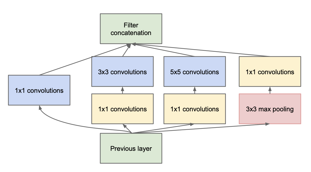 **Figure 5:** Diagram of an Inception Module (with dimension reduction) ([Szegedy et al., "Going deeper with convolutions," 2015](https://arxiv.org/abs/1409.4842))
**Number of Parameters**
Before applying the $ 3 \times 3 $ and $ 5 \times 5 $ convolutions, a $ 1 \times 1 $ convolution reduces the number of channels to a chosen value determined by the number of $ 1 \times 1 $ filters.
If the $ 1 \times 1 $ layer has $ F_1 $ filters and the $ 3 \times 3 $ or $ 5 \times 5 $ layer has $ F_2 $ filters, then
* $ 3\times 3 $ convolution: $ 3 \times 3 \times F_1 \times F_2 $ parameters
* $ 5 \times 5 $ convolution: $ 5 \times 5 \times F_1 \times F_2 $ parameters
The key here is that *we can choose* $ F_1 $ to reduce the parameter counts.
**Number of Channels**
After max pooling, a $ 1 \times 1 $ convolution is used to reduce the number of channels before concatenation. This limits the number of output channels from this module and, thus, the number of parameters in subsequent modules.
### GoogLeNet Architecture
The full GoogLeNet architecture uses a series of Inception Modules stacked together:
**Figure 5:** Diagram of an Inception Module (with dimension reduction) ([Szegedy et al., "Going deeper with convolutions," 2015](https://arxiv.org/abs/1409.4842))
**Number of Parameters**
Before applying the $ 3 \times 3 $ and $ 5 \times 5 $ convolutions, a $ 1 \times 1 $ convolution reduces the number of channels to a chosen value determined by the number of $ 1 \times 1 $ filters.
If the $ 1 \times 1 $ layer has $ F_1 $ filters and the $ 3 \times 3 $ or $ 5 \times 5 $ layer has $ F_2 $ filters, then
* $ 3\times 3 $ convolution: $ 3 \times 3 \times F_1 \times F_2 $ parameters
* $ 5 \times 5 $ convolution: $ 5 \times 5 \times F_1 \times F_2 $ parameters
The key here is that *we can choose* $ F_1 $ to reduce the parameter counts.
**Number of Channels**
After max pooling, a $ 1 \times 1 $ convolution is used to reduce the number of channels before concatenation. This limits the number of output channels from this module and, thus, the number of parameters in subsequent modules.
### GoogLeNet Architecture
The full GoogLeNet architecture uses a series of Inception Modules stacked together:
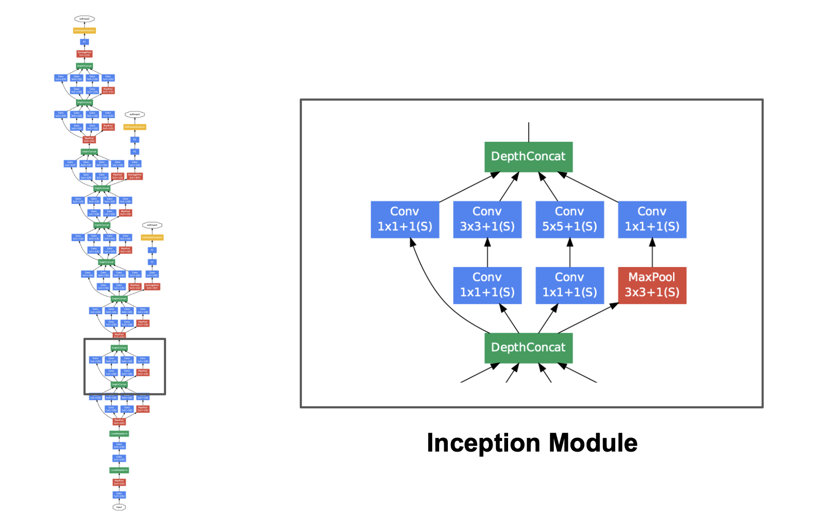 **Figure 6:** The full GoogLeNet architecture, a series of Inception modules ([Szegedy et al., "Going deeper with convolutions," 2015](https://arxiv.org/abs/1409.4842))
GoogLeNet showed that deep networks can perform well while keeping parameter counts under control. It also introduced auxiliary classifiers during training to help mitigate the vanishing gradient problem (see the original paper [here](https://arxiv.org/pdf/1409.4842)).
However, as researchers worked toward even deeper networks, optimization difficulties and vanishing gradients remained significant challenges. This limitation led to the development of Residual Networks (ResNets), which address gradient flow more directly via skip connections.
## ResNets
Short for Residual Networks, ResNets were introduced by He et al. in 2015 to solve a counterintuitive problem: as networks get deeper, accuracy often plateaus and then degrades rapidly. This isn't just due to overfitting; even training error becomes higher in very deep "plain" networks.
The main innovation of ResNets is the residual block, where the input is passed directly to a deeper layer, skipping one or more layers in between.
A basic **residual block** consists of:
1. **Two convolutional layers**, and
2. A **skip connection** that bypasses these layers and adds the input directly to the output.
**Figure 6:** The full GoogLeNet architecture, a series of Inception modules ([Szegedy et al., "Going deeper with convolutions," 2015](https://arxiv.org/abs/1409.4842))
GoogLeNet showed that deep networks can perform well while keeping parameter counts under control. It also introduced auxiliary classifiers during training to help mitigate the vanishing gradient problem (see the original paper [here](https://arxiv.org/pdf/1409.4842)).
However, as researchers worked toward even deeper networks, optimization difficulties and vanishing gradients remained significant challenges. This limitation led to the development of Residual Networks (ResNets), which address gradient flow more directly via skip connections.
## ResNets
Short for Residual Networks, ResNets were introduced by He et al. in 2015 to solve a counterintuitive problem: as networks get deeper, accuracy often plateaus and then degrades rapidly. This isn't just due to overfitting; even training error becomes higher in very deep "plain" networks.
The main innovation of ResNets is the residual block, where the input is passed directly to a deeper layer, skipping one or more layers in between.
A basic **residual block** consists of:
1. **Two convolutional layers**, and
2. A **skip connection** that bypasses these layers and adds the input directly to the output.
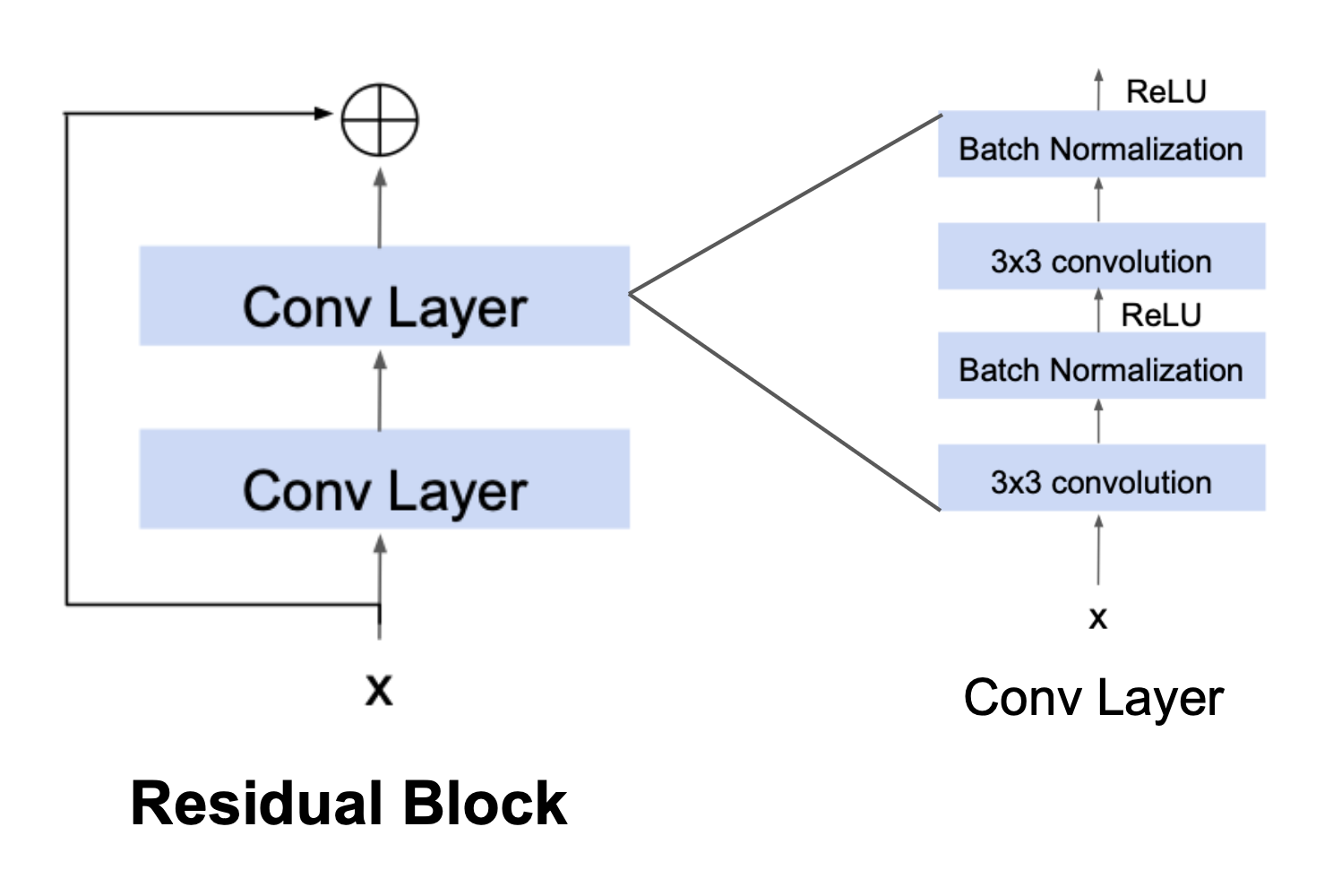 **Figure 7:** A residual block (left), the main component of a ResNet; see how the input $ x $ is added element-wise to the output of the block ([CS 4782, Cornell University, 2026](https://www.cs.cornell.edu/courses/cs4782/2026sp/slides/pdf/week4_1_complete.pdf))
> **Note:** As above, a convolutional layer will now refer to a series of convolution, batch normalization, and ReLU layers.
These residual blocks connected together create the ResNet. This architecture solves two main problems which lead to higher training error in deep "plain" networks:
1. **Vanishing Gradients:** The skip connection provides a direct path for the gradient to flow through the network during backpropagation. This prevents small gradients ($ < 1 $) from being repeatedly multiplied together and diminishing to $ 0 $.
2. **Residual Learning:** By passing the input $ x $ forward unchanged, the stacked layers only need to learn the **residual** mapping (the difference) required to reach the target output, which is an easier optimization problem. That is, the identity mapping propagates features from earlier blocks, so convolutional layers focus on learning refinements to the representation rather than preserving existing features.
### Backpropagation
To emphasize how ResNets address the vanishing gradient problem, below we compare backpropagation through regular convolutional layers vs. residual blocks.
#### Backprop Through Regular Convolution Layers
When backpropagating through "plain" convolutional layers, we chain the gradient calculation:
**Figure 7:** A residual block (left), the main component of a ResNet; see how the input $ x $ is added element-wise to the output of the block ([CS 4782, Cornell University, 2026](https://www.cs.cornell.edu/courses/cs4782/2026sp/slides/pdf/week4_1_complete.pdf))
> **Note:** As above, a convolutional layer will now refer to a series of convolution, batch normalization, and ReLU layers.
These residual blocks connected together create the ResNet. This architecture solves two main problems which lead to higher training error in deep "plain" networks:
1. **Vanishing Gradients:** The skip connection provides a direct path for the gradient to flow through the network during backpropagation. This prevents small gradients ($ < 1 $) from being repeatedly multiplied together and diminishing to $ 0 $.
2. **Residual Learning:** By passing the input $ x $ forward unchanged, the stacked layers only need to learn the **residual** mapping (the difference) required to reach the target output, which is an easier optimization problem. That is, the identity mapping propagates features from earlier blocks, so convolutional layers focus on learning refinements to the representation rather than preserving existing features.
### Backpropagation
To emphasize how ResNets address the vanishing gradient problem, below we compare backpropagation through regular convolutional layers vs. residual blocks.
#### Backprop Through Regular Convolution Layers
When backpropagating through "plain" convolutional layers, we chain the gradient calculation:
 $$\frac{\partial \mathcal{L}}{\partial \mathbf{a}} =\frac{\partial \mathcal{L}}{\partial \mathbf{z}}\frac{\partial \mathbf{z}}{\partial \mathbf{a}} = \frac{\partial \mathcal{L}}{\partial \mathbf{z}}(F'(\mathbf{a}))$$
#### Backprop Through Residual Blocks
Notice the difference when we calculate the gradient for the residual block:
$$\frac{\partial \mathcal{L}}{\partial \mathbf{a}} =\frac{\partial \mathcal{L}}{\partial \mathbf{z}}\frac{\partial \mathbf{z}}{\partial \mathbf{a}} = \frac{\partial \mathcal{L}}{\partial \mathbf{z}}(F'(\mathbf{a}))$$
#### Backprop Through Residual Blocks
Notice the difference when we calculate the gradient for the residual block:
 $$\frac{\partial \mathcal{L}}{\partial \mathbf{a}} =\frac{\partial \mathcal{L}}{\partial \mathbf{z}}\frac{\partial \mathbf{z}}{\partial \mathbf{a}} = \frac{\partial \mathcal{L}}{\partial \mathbf{z}}(F'(\mathbf{a})+1)$$
Since we have added $ \mathbf{a} $ to the output $ F(\mathbf{a}) $, our computation of $ \frac{\partial \mathbf{z}}{\partial \mathbf{a}} $ gains a $ +1 $. This addition helps alleviate vanishing gradients, because even if $ F'(\mathbf{a}) $ is small, the $ +1 $ boosts the value of the gradient away from $ 0 $.
### ResNet Architecture
To create the actual ResNet architecture, we combine several residual blocks by using the output of the previous block as input to the next one:
$$\frac{\partial \mathcal{L}}{\partial \mathbf{a}} =\frac{\partial \mathcal{L}}{\partial \mathbf{z}}\frac{\partial \mathbf{z}}{\partial \mathbf{a}} = \frac{\partial \mathcal{L}}{\partial \mathbf{z}}(F'(\mathbf{a})+1)$$
Since we have added $ \mathbf{a} $ to the output $ F(\mathbf{a}) $, our computation of $ \frac{\partial \mathbf{z}}{\partial \mathbf{a}} $ gains a $ +1 $. This addition helps alleviate vanishing gradients, because even if $ F'(\mathbf{a}) $ is small, the $ +1 $ boosts the value of the gradient away from $ 0 $.
### ResNet Architecture
To create the actual ResNet architecture, we combine several residual blocks by using the output of the previous block as input to the next one:
 **Figure 8:** Chaining residual blocks together to form a ResNet.
Compare this to a traditional, "Plain" CNN, which has no skip connections:
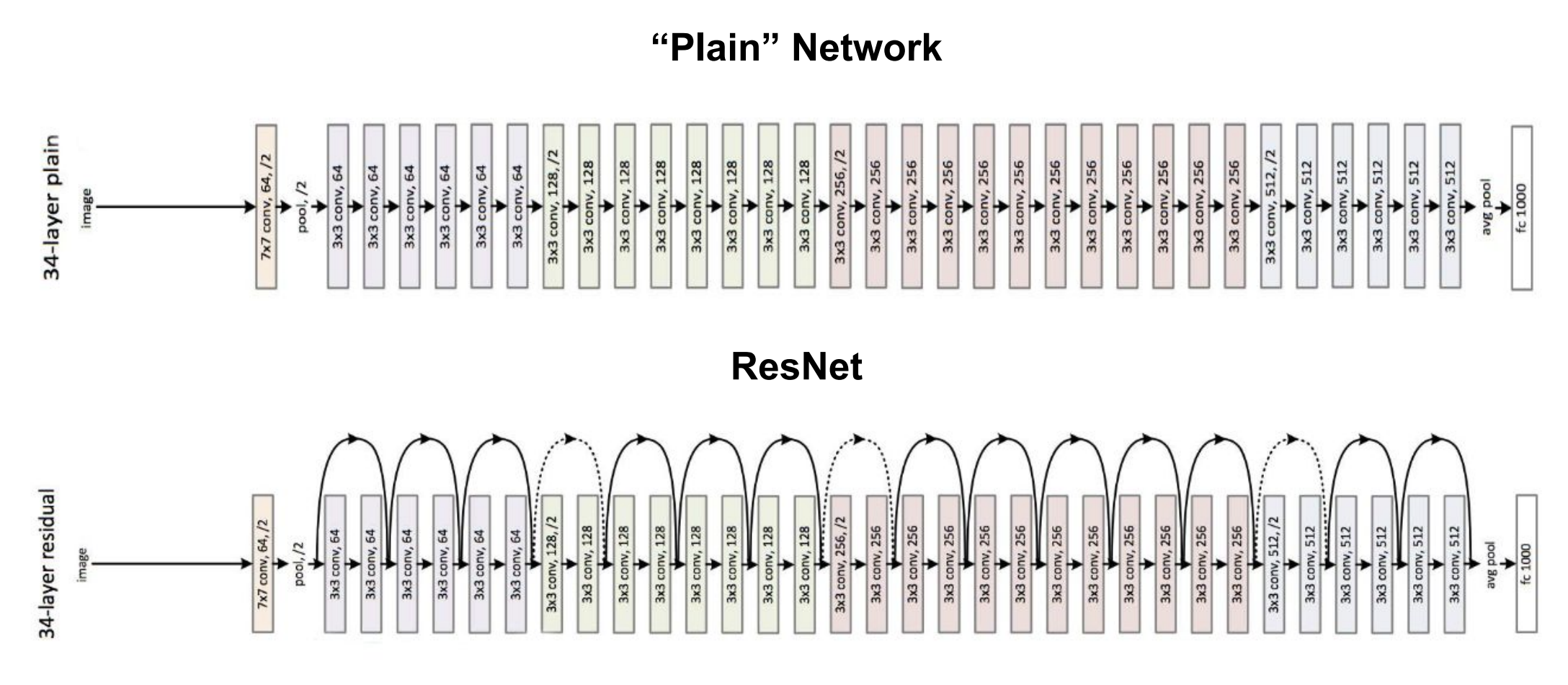
**Figure 9:** The architecture of a deep "plain" CNN vs. a ResNet, which has skip connections in the residual blocks ([He et al., "Deep residual learning for image recognition," 2016](https://arxiv.org/abs/1512.03385))
With multiple residual blocks stacked together, we can have a much deeper ResNet that solves the problem of the vanishing gradients we encountered in the deep CNNs.
### Now: Deeper == Better
"Plain" deep networks (counterintuitively) struggled with optimization difficulties and underfitting, causing them to have a higher error rate than their shallower counterparts.
ResNets address this issue: in the example below, the deeper $ 34 $-layer ResNet achieves a lower training and validation error than the $ 18 $-layer ResNet.
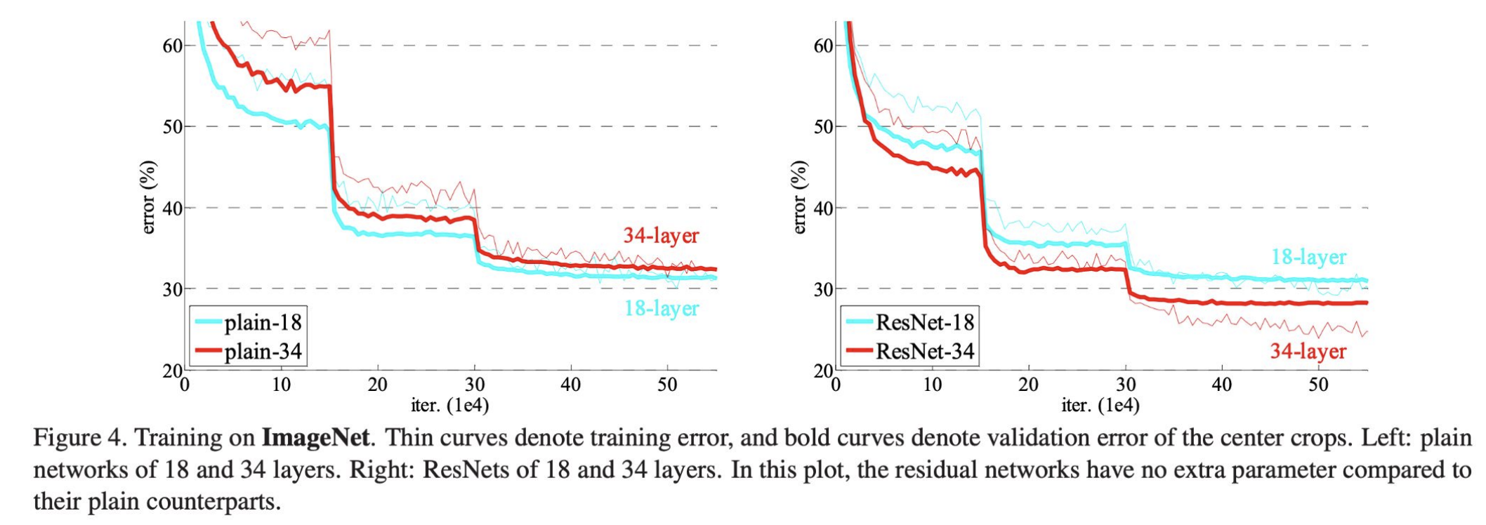
**Figure 10:** Training error for $ 34 $-layer vs. $ 18 $-layer "plain" CNNs (left) and ResNets (right). Unlike with the "plain" CNNs, the deeper ResNet has a lower training error ([He et al., "Deep residual learning for image recognition," 2016](https://arxiv.org/abs/1512.03385))
Unlike plain CNNs, increasing a ResNet's depth generally improves performance rather than harming it.
Another advantage of residual connections—aside from improving gradient flow and enabling residual learning—is that they smooth out the loss landscape:
**Figure 8:** Chaining residual blocks together to form a ResNet.
Compare this to a traditional, "Plain" CNN, which has no skip connections:

**Figure 9:** The architecture of a deep "plain" CNN vs. a ResNet, which has skip connections in the residual blocks ([He et al., "Deep residual learning for image recognition," 2016](https://arxiv.org/abs/1512.03385))
With multiple residual blocks stacked together, we can have a much deeper ResNet that solves the problem of the vanishing gradients we encountered in the deep CNNs.
### Now: Deeper == Better
"Plain" deep networks (counterintuitively) struggled with optimization difficulties and underfitting, causing them to have a higher error rate than their shallower counterparts.
ResNets address this issue: in the example below, the deeper $ 34 $-layer ResNet achieves a lower training and validation error than the $ 18 $-layer ResNet.

**Figure 10:** Training error for $ 34 $-layer vs. $ 18 $-layer "plain" CNNs (left) and ResNets (right). Unlike with the "plain" CNNs, the deeper ResNet has a lower training error ([He et al., "Deep residual learning for image recognition," 2016](https://arxiv.org/abs/1512.03385))
Unlike plain CNNs, increasing a ResNet's depth generally improves performance rather than harming it.
Another advantage of residual connections—aside from improving gradient flow and enabling residual learning—is that they smooth out the loss landscape:
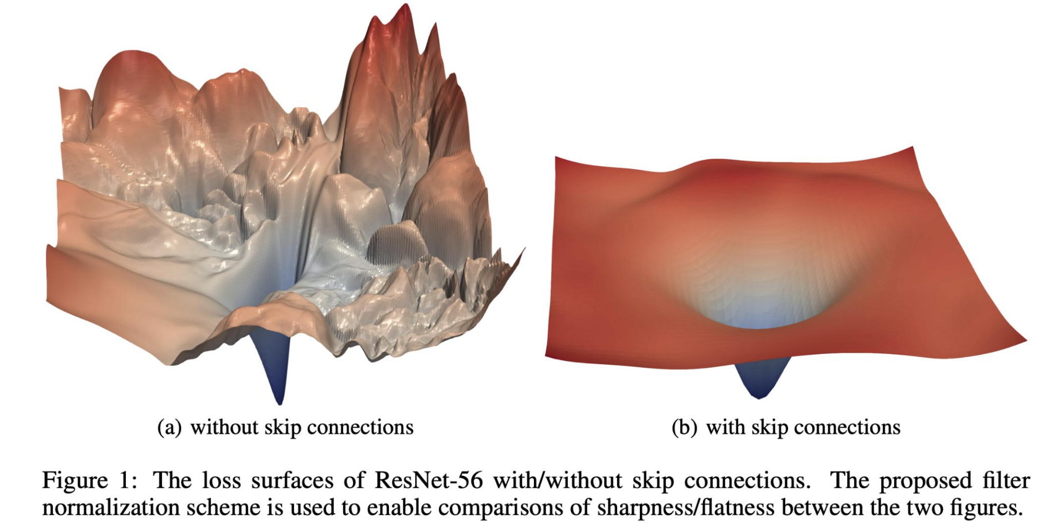 **Figure 11:** Loss surfaces of a network without (left) vs. with (right) skip connections. ([Li et al., "Visualizing the loss landscape of neural nets," 2018](https://arxiv.org/abs/1712.09913))
These properties make ResNets easier to optimize than plain CNNs, allowing deeper architectures to fully leverage additional layers.
Even with these improvements, though, training deep CNNs can still be a long and computationally expensive process. This motivates techniques like stochastic depth.
## Stochastic Depth
**Stochastic depth** is a training technique that randomly "drops" residual blocks—similar to dropout, but with entire residual blocks instead of individual neurons.
**Figure 11:** Loss surfaces of a network without (left) vs. with (right) skip connections. ([Li et al., "Visualizing the loss landscape of neural nets," 2018](https://arxiv.org/abs/1712.09913))
These properties make ResNets easier to optimize than plain CNNs, allowing deeper architectures to fully leverage additional layers.
Even with these improvements, though, training deep CNNs can still be a long and computationally expensive process. This motivates techniques like stochastic depth.
## Stochastic Depth
**Stochastic depth** is a training technique that randomly "drops" residual blocks—similar to dropout, but with entire residual blocks instead of individual neurons.
 **Figure 12:** Visualization of stochastic depth during training, where the middle residual block is dropped.
Stochastic depth has two key benefits:
1. **Computation Savings:** We train smaller subnetworks, saving on computation and shortening training time.
2. **Improved Generalization:** Randomly removing residual blocks effectively creates an ensemble effect, improving performance on unseen data.
### Training vs. Testing
During **training**, each residual block is kept with probability $ p $, the "survival probability." Dropping residual blocks during training means those blocks are not part of the forward or the backward pass, saving computation.
This makes $ p $ is a key hyperparameter of the model, raising the question of how to choose it. In the paper "Deep networks with stochastic depth," Huang et al. found success with a linear decay of $ p $ throughout the network. Specifically, this meant setting the survival rate $ p_{\ell} $ for layer $ \ell \in \{1, 2, ..., L\} $ as
$$p_{\ell} = 1 - \frac{\ell}{L}(1-p_L) $$
where $ p_L $ is the survival probability for the last layer. With this formulation, residual blocks later in the network are more likely to be dropped.
**Figure 12:** Visualization of stochastic depth during training, where the middle residual block is dropped.
Stochastic depth has two key benefits:
1. **Computation Savings:** We train smaller subnetworks, saving on computation and shortening training time.
2. **Improved Generalization:** Randomly removing residual blocks effectively creates an ensemble effect, improving performance on unseen data.
### Training vs. Testing
During **training**, each residual block is kept with probability $ p $, the "survival probability." Dropping residual blocks during training means those blocks are not part of the forward or the backward pass, saving computation.
This makes $ p $ is a key hyperparameter of the model, raising the question of how to choose it. In the paper "Deep networks with stochastic depth," Huang et al. found success with a linear decay of $ p $ throughout the network. Specifically, this meant setting the survival rate $ p_{\ell} $ for layer $ \ell \in \{1, 2, ..., L\} $ as
$$p_{\ell} = 1 - \frac{\ell}{L}(1-p_L) $$
where $ p_L $ is the survival probability for the last layer. With this formulation, residual blocks later in the network are more likely to be dropped.
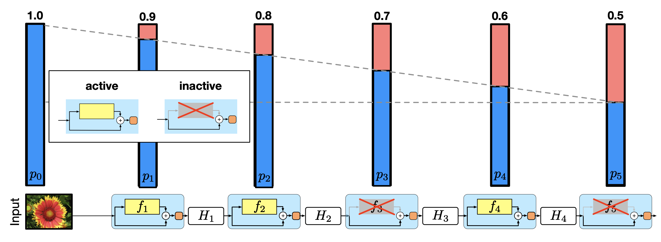 **Figure 13:** Linear decay of the survival probability with depth ([Huang et al., "Deep networks with stochastic depth," 2016](https://arxiv.org/abs/1603.09382))
During **testing**, all residual blocks are active, and their outputs are scaled by their survival probability to match the expected activations during training.
While ResNets trained with stochastic depth typically have a higher training loss, their *test error* is lower. Training with stochastic depth essentially trains an ensemble network, which mitigates overfitting and helps the model generalize to unseen data.
## DenseNets
DenseNets (Dense Convolutional Networks), introduced by [Huang et al. in 2017](https://arxiv.org/pdf/1608.06993), extend the idea of residual connections by *concatenating* each layers output to the inputs of all subsequent layers within a dense block.
### Dense Blocks
Dense blocks are the main building block of DenseNets. Whereas residual blocks add the input to the output, dense blocks *concatenate* the input to the output:
**Figure 13:** Linear decay of the survival probability with depth ([Huang et al., "Deep networks with stochastic depth," 2016](https://arxiv.org/abs/1603.09382))
During **testing**, all residual blocks are active, and their outputs are scaled by their survival probability to match the expected activations during training.
While ResNets trained with stochastic depth typically have a higher training loss, their *test error* is lower. Training with stochastic depth essentially trains an ensemble network, which mitigates overfitting and helps the model generalize to unseen data.
## DenseNets
DenseNets (Dense Convolutional Networks), introduced by [Huang et al. in 2017](https://arxiv.org/pdf/1608.06993), extend the idea of residual connections by *concatenating* each layers output to the inputs of all subsequent layers within a dense block.
### Dense Blocks
Dense blocks are the main building block of DenseNets. Whereas residual blocks add the input to the output, dense blocks *concatenate* the input to the output:
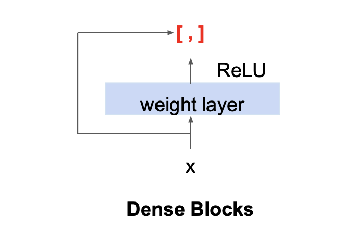 **Figure 14:** A layer within a dense block, the fundamental building block of a DenseNet; $ [ \ ,\ ] $ denotes concatenation ([CS 4782, Cornell University, 2026](https://www.cs.cornell.edu/courses/cs4782/2026sp/slides/pdf/week4_1_complete.pdf))
Due to this concatenation, the number of *input* channels to each layer increases as we progress through the layers of a dense block:
**Figure 14:** A layer within a dense block, the fundamental building block of a DenseNet; $ [ \ ,\ ] $ denotes concatenation ([CS 4782, Cornell University, 2026](https://www.cs.cornell.edu/courses/cs4782/2026sp/slides/pdf/week4_1_complete.pdf))
Due to this concatenation, the number of *input* channels to each layer increases as we progress through the layers of a dense block:
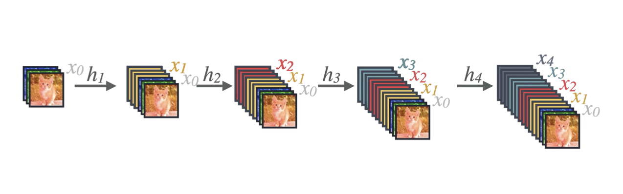 **Figure 15:** Growth of the **input** channels by $ k=3 $ to each layer within a dense block ([CS 4782, Cornell University, 2026](https://www.cs.cornell.edu/courses/cs4782/2026sp/slides/pdf/week4_1_complete.pdf))
The rate at which the number of input channels increases within a dense block is a hyperparameter $ k $, the growth rate. If each layer $ \ell $ outputs $ k $ feature maps, the $ \ell $-th layer of the dense block will have
$$ k_0 + k \times (\ell -1) $$
input channels, where $ k_0 $ is the number of input channels to the block. Huang et al. found that relatively small values of $ k $, for example $ k=12 $, proved effective in DenseNets.
Keep in mind that each layer only outputs $ k $ feature maps, one from each of its $ k $ filters; a more complete picture of a dense block is shown below:
**Figure 15:** Growth of the **input** channels by $ k=3 $ to each layer within a dense block ([CS 4782, Cornell University, 2026](https://www.cs.cornell.edu/courses/cs4782/2026sp/slides/pdf/week4_1_complete.pdf))
The rate at which the number of input channels increases within a dense block is a hyperparameter $ k $, the growth rate. If each layer $ \ell $ outputs $ k $ feature maps, the $ \ell $-th layer of the dense block will have
$$ k_0 + k \times (\ell -1) $$
input channels, where $ k_0 $ is the number of input channels to the block. Huang et al. found that relatively small values of $ k $, for example $ k=12 $, proved effective in DenseNets.
Keep in mind that each layer only outputs $ k $ feature maps, one from each of its $ k $ filters; a more complete picture of a dense block is shown below:
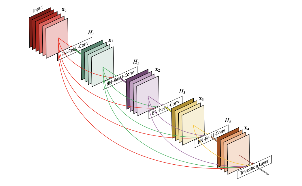 **Figure 16:** A five-layer dense block with growth rate $ k=4 $ ([Huang et al., "Densely Connected Convolutional Networks", 2017](https://arxiv.org/pdf/1608.06993))
Connecting these dense blocks together gives us a DenseNet.
### DenseNet Architecture
A full DenseNet consists of dense blocks separated by transition layers. A transition layer includes $ 1 \times 1 $ convolution and pooling to control feature map size, as well as batch normalization.
**Figure 16:** A five-layer dense block with growth rate $ k=4 $ ([Huang et al., "Densely Connected Convolutional Networks", 2017](https://arxiv.org/pdf/1608.06993))
Connecting these dense blocks together gives us a DenseNet.
### DenseNet Architecture
A full DenseNet consists of dense blocks separated by transition layers. A transition layer includes $ 1 \times 1 $ convolution and pooling to control feature map size, as well as batch normalization.
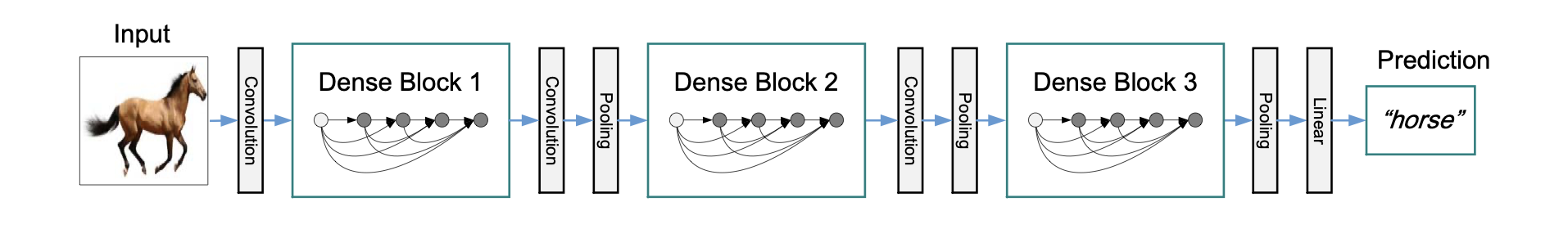 **Figure 17:** A DenseNet with three dense blocks and transition layers between blocks ([Huang et al., "Densely Connected Convolutional Networks", 2017](https://arxiv.org/pdf/1608.06993))
The dense block architecture has several benefits in terms of training and performance. Since each layer has access to the outputs of all previous layers, we witness:
1. **Fewer parameters:** DenseNets actually require fewer parameters than traditional CNNs because they do not have to learn redundant feature maps. Recall that $ k $ is relatively small, and concatenating outputs allows for feature map reuse.
2. **Information flow:** Like ResNets, DenseNets emphasize information flow through the network, with each layer having access to the "collective knowledge" of the network.
3. **Addressing vanishing gradients:** DenseNets alleviate the vanishing gradient problem: the concatenation architecture provides many "short" paths back to earlier weights, so we don't have long chains of derivatives during backpropagation.
DenseNets maximize feature reuse and strengthen gradient flow, enabling deep networks to train efficiently while maintaining parameter efficiency.
## Summary
Deep CNNs generally outperform shallow networks because they are able to capture more complex relationships. However, increasing depth makes optimization more difficult, often leading to higher training error, vanishing gradients, and longer training times.
Architectural innovations like **GoogLeNet**, **ResNets**, and **DenseNets** address these challenges. Inception modules (GoogLeNet) control parameter growth through dimension reduction, while residual and dense connections improve gradient flow and make deep networks easier to optimize. Additionally, **stochastic depth** speeds up training and improves generalization by randomly dropping residual blocks during training.
### Summary of CNN Architectures
“Plain” CNN | GoogLeNet | ResNet | DenseNet |
| :---: | :---: | :---: | :---: |
| Simple connection from previous to next layer | $ 1\times 1 $, $ 3\times 3 $, and $ 5\times 5 $ convolutions and pooling between each layer | Skip connections: add output of previous layer to next layer | Dense connections: concatenate output of previous layers to next layer |
|  | |  |  |
These advances are key developments in modern CNN architectures, making it practical to train deep networks effectively.
**Figure 17:** A DenseNet with three dense blocks and transition layers between blocks ([Huang et al., "Densely Connected Convolutional Networks", 2017](https://arxiv.org/pdf/1608.06993))
The dense block architecture has several benefits in terms of training and performance. Since each layer has access to the outputs of all previous layers, we witness:
1. **Fewer parameters:** DenseNets actually require fewer parameters than traditional CNNs because they do not have to learn redundant feature maps. Recall that $ k $ is relatively small, and concatenating outputs allows for feature map reuse.
2. **Information flow:** Like ResNets, DenseNets emphasize information flow through the network, with each layer having access to the "collective knowledge" of the network.
3. **Addressing vanishing gradients:** DenseNets alleviate the vanishing gradient problem: the concatenation architecture provides many "short" paths back to earlier weights, so we don't have long chains of derivatives during backpropagation.
DenseNets maximize feature reuse and strengthen gradient flow, enabling deep networks to train efficiently while maintaining parameter efficiency.
## Summary
Deep CNNs generally outperform shallow networks because they are able to capture more complex relationships. However, increasing depth makes optimization more difficult, often leading to higher training error, vanishing gradients, and longer training times.
Architectural innovations like **GoogLeNet**, **ResNets**, and **DenseNets** address these challenges. Inception modules (GoogLeNet) control parameter growth through dimension reduction, while residual and dense connections improve gradient flow and make deep networks easier to optimize. Additionally, **stochastic depth** speeds up training and improves generalization by randomly dropping residual blocks during training.
### Summary of CNN Architectures
“Plain” CNN | GoogLeNet | ResNet | DenseNet |
| :---: | :---: | :---: | :---: |
| Simple connection from previous to next layer | $ 1\times 1 $, $ 3\times 3 $, and $ 5\times 5 $ convolutions and pooling between each layer | Skip connections: add output of previous layer to next layer | Dense connections: concatenate output of previous layers to next layer |
|  | |  |  |
These advances are key developments in modern CNN architectures, making it practical to train deep networks effectively.