Word Embeddings

# CS4782: Word Embeddings
## Introduction
Previously, we have been looking at image models. These include:
* **CNN**
* Basic convolutional architecture that can capture local spatial patterns using sequential convolutional layers
* **GoogleNet**
* Uses multiple convolutions for each layer – 1x1, 3x3, 5x5, max pooling
* Concatenates these individual results into the input for the next layer
* 1x1 convolutions address the vanishing gradient problem, which proved critical in the performance of this model
* Typically, each filter results in fewer output channels with an additional helper 1x1 convolution, allowing for concatenation to roughly preserve the number of channels from layer to layer
* **ResNet**
* Layer $ (i+1) $ is the input to layer $ (i) $ added to the output of layer $ (i) $
* Mathematically, $ z = x + F(x) $
* Therefore, $ \frac{dz}{dx} = 1 + F'(x) $
* This $ +1 $ “keeps the gradient alive” (handles vanishing gradient problem), allowing deeper networks to be trained
* If $ z = F(x) $: $ \frac{dz}{dx} = F'(x) $, and gradient may vanish
* **DenseNet**
* Every previous output channel is concatenated before the input to the next layer
* Therefore, if a layer has $ k $ filters, the number of channels strictly increases by $ k $ from that layer to the next
* Promotes feature reuse and improves gradient flow
Handling text data brings in a new set of complexities!
* **Homonyms**
* I swung the baseball bat / I saw a bat in the cave
* **Typos / missing words / incorrect spelling**
* I _ around the track
* This past weak has been very difficult.
* **Paraphrases and synonyms**
* I saw my dad / I spent time with my father
* **Switching word order results in different meaning**
* The man hit the woman / The woman hit the man
All of this indicates we will need more complexities (including accounting for word ordering) when handling text.
---
## Model 1: n-Gram
Our goal is to assign probabilities to text; given a sequence $ (x_1, x_2, \ldots, x_n) $, maximize its probability
$ P(x_1, x_2, \ldots, x_n) $. By the chain rule of statistics:
$$
P(x_1, x_2, \ldots, x_n) =
P(x_1)P(x_2|x_1)P(x_3|x_2, x_1)\ldots P(x_n|x_1, x_2, \ldots, x_{n-1})
$$
Looking at the individual terms, we are attempting to maximize the probability of the next word, given what we have seen so far.
In n-Gram models, we are simply looking at chunks of words, and finding the most common word that could come next:
* **Uni-gram**: looks at the previous 0 words (so each word is predicted individually)
* **Bi-gram**: looks at the previous word (finding the most common clump of 2 beginning with that word)
* **Tri-gram**: looks at the previous 2 words
Mathematically,
$$
P(x_t|x_1, x_2, \ldots, x_{t-1}) =
\frac{\text{count}(x_{t-n+1}, \ldots, x_{t-1}, x_t)}
{\text{count}(x_{t-n+1}, \ldots, x_{t-1})}
$$
Where in uni-gram $ n=1 $, bi-gram $ n=2 $, tri-gram $ n=3 $.
**Increasing $ n $?**
* **Pro**: We take in more contextual information. In fact if $ n=1 $, we are not even considering prior words!
* **Con**: We need to store much much more memory. If $ n=3 $, we need to store the counts of all 3-word sequences, which takes $ V^3 $ space (if $ V $ = vocab size)
* Exponential scaling in terms of $ n $
---
## Tokenization
Before any model can process text, we must decide **how to split raw text into discrete units**, called *tokens*. This step is known as **tokenization**, and it has a large impact on both model performance and computational efficiency.
Key questions when tokenizing text include:
* How large should the vocabulary be?
* Should tokens correspond to **words**, **subwords**, or **characters**?
* How should we handle rare or unseen words?
A simple word-level vocabulary can grow extremely large and fails to generalize to unseen words. Character-level tokenization avoids this issue but produces very long sequences and loses semantic structure.
Modern NLP systems typically use **subword tokenization**, which balances vocabulary size and expressiveness.
### Byte-Pair Encoding (BPE)
Byte-Pair Encoding starts with individual characters and repeatedly merges the most frequently occurring adjacent token pairs. Over time, common word fragments (e.g., “ing”, “tion”) become single tokens.
Demo [here](https://www.cs.cornell.edu/courses/cs4782/2026sp/demos/bytepair/) (shown in lecture) is a step-by-step visualization of how subword tokenizers are learned and applied. We start with a character-level representation and then gradually pair the most frequent adjacent symbols, eventually merging them to form a growing subword vocabulary.
### WordPiece
WordPiece is a variant of BPE that chooses merges based on maximizing the likelihood of the training data. It is commonly used in Transformer models such as BERT.
Subword tokenization allows models to:
* Represent rare or unseen words
* Share meaning across related words (e.g., *run*, *running*, *runner*)
* Keep vocabularies manageable while preserving semantic structure
---
## Bag of Words
Store the words of the text and their count / quantity (essentially, keeping track of how much of each “item” we have in our bag).
This is good for a basic representation of text, but:
* Doesn’t take word ordering into account (which can easily impact meaning)
* We do not even know which words were next to each other
* Doesn’t capture meaning or relationships between words
* Results in a high-dimensional vector – one feature for each word
* Very similar text can have completely different bag of words representations (if synonyms / paraphrases used)
There are better ways to represent text!
---
## Word Embeddings
The idea is to represent each word as a vector. Formally, let there be a set of words $ V $, and a set of features $ F $.
$ F $ are characteristics of words; “human”, or “female”, or “plural”, etc.
Then, for each $ i \in V $, define the semantic representation as $ x_i $. Each $ x_i $ is an $ F $-dimensional vector, where $ x_{if} $ represents the value of word $ i $ on feature $ f $.
We learn a lot about words from these vectors:
* Similarity / difference, which can be measured by vector distance; cosine similarity
* “Strongest” features for particular words
* Words can be mapped to an embedding space, capturing semantic relationships
Once we have numerical representations of words, we can use these for a variety of word prediction tasks.
**Similar words appear in similar contexts!**
If words $ i, i' $ have similar vector representations, chances are their surrounding words will often be similar. In essence – we are looking for word vectors that inform the surrounding context.
---
## Training Task 1: Skip-Gram
Goal: given a target word, predict surrounding context words.
Formally, create a probability distribution of observing context words given a target word, and maximize these probabilities for surrounding words.
Suppose we have the sentence “I drank green tea this morning”, where *tea* is our target word. We are trying to maximize:
$$
P(\text{drank}|\text{tea}),\;
P(\text{green}|\text{tea}),\;
P(\text{this}|\text{tea}),\;
P(\text{morning}|\text{tea})
$$
Define a matrix $ W \in \mathbb{R}^{|V| \times D} $. This matrix represents the $ D $-dimensional embeddings for each word in $ V $.
The probability is:
$$
P(w_c|w_t) =
\frac{\exp(W_t W_c^T)}{\sum_i \exp(W_t W_i^T)}
$$
The loss function is cross-entropy:
$$
L_\theta = -\log P(w_c|w_t)
$$
### word2vec
Word2Vec is a family of models for learning vector representations of words directly from raw text. The core idea is simple: a word is defined by the context of the words around it. In the Skip-gram variant, the model is shown a target word and asked to predict the surrounding context words, forcing the learned vectors to encode semantic and syntactic relationships. Over many examples, words that appear in similar contexts (e.g., “coffee” and “tea”) end up with similar embeddings, enabling downstream models to reason about meaning using continuous vector representations rather than discrete word IDs.
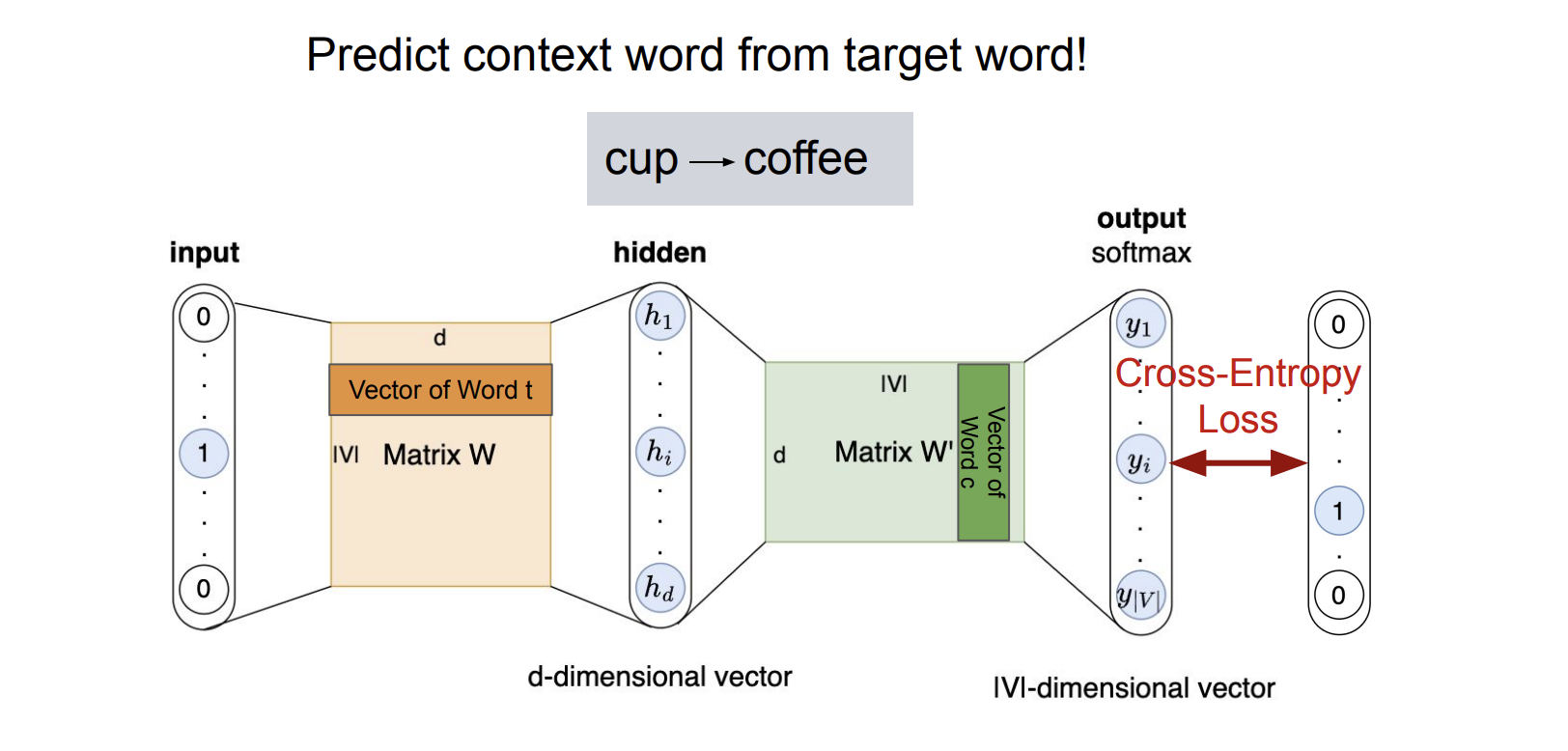
In the Skip-gram Word2Vec model, training proceeds by treating each word in a corpus as a target and learning to predict its surrounding context words. The input is a one-hot encoding of the target word, which, when multiplied by the embedding matrix W, simply selects the corresponding word vector (the word’s embedding). This embedding is then projected through a second matrix W' to produce scores over the entire vocabulary, which are converted into a probability distribution with a softmax. The model is trained to maximize the likelihood of the true context words given the target word, updating both W and W' via gradient descent. In practice, this full softmax is often approximated with techniques like negative sampling or hierarchical softmax to make training scalable to large vocabularies.
## Training Task 2: Continuous Bag of Words (CBOW)
**Goal:** The Continuous Bag of Words (CBOW) model learns word embeddings by **predicting a target (center) word from its surrounding context words**. Given a window of size $ m $, the model observes the context $ (w_{t-m}, \ldots, w_{t-1}, w_{t+1}, \ldots, w_{t+m}) $ and aims to predict the missing middle word $ w_t $. For example, in the sentence *“A cup of coffee is on the table”*, the context $ (\text{cup}, \text{of}, \text{is}, \text{on}) $ is used to predict the target word *coffee*, as illustrated in the figure.
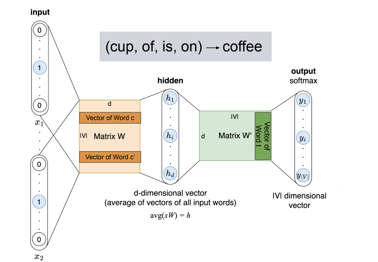
**Model architecture.**
Each context word is represented as a one-hot vector and mapped to a dense embedding via the shared embedding matrix $ W $. The embeddings of all context words are then **averaged** to produce a single $ d $-dimensional hidden vector:
$$h = \text{avg}(xW)$$
where \(x\) denotes the set of one-hot inputs for the context words. This aggregated context representation is passed through a second matrix \(W'\) to produce a score for every word in the vocabulary. A softmax over these scores yields a probability distribution over possible target words.
**Training objective.**
The model is trained to maximize the likelihood of the true center word given its context:
$$L_\theta = -\log P(w_t \mid w_{t-m}, \ldots, w_{t+m})$$
**Intuition and comparison to Skip-gram.**
CBOW can be viewed as “smoothing” information from multiple surrounding words to infer the missing center word. Because it aggregates context into a single averaged vector, CBOW is computationally efficient and stable on large corpora. However, this averaging can blur fine-grained distinctions and makes CBOW less sensitive to rare words compared to Skip-gram, which predicts each context word individually from the target. In practice, CBOW often learns strong representations for frequent words, while Skip-gram tends to perform better on infrequent or specialized vocabulary.
---
## Word Mover’s Distance
* A similarity metric between documents
* The minimum distance needed to match all words from one document to the other
---
## X2Vec Approaches
The embedding approach has been extended to other data types:
* Word2Vec
* Doc2Vec
* Node2Vec
* Item2Vec
* Sent2Vec
---
## Word2Vec Characteristics and Limitations
* Word embeddings are time-dependent as the meaning of words can change over time
* Word embeddings can inherit societal biases present in the training data
* Each word has one representation, even if there is multiple meaning for the word
* Words are trained within a context window, which may not capture broader relationships
---
## RNNs
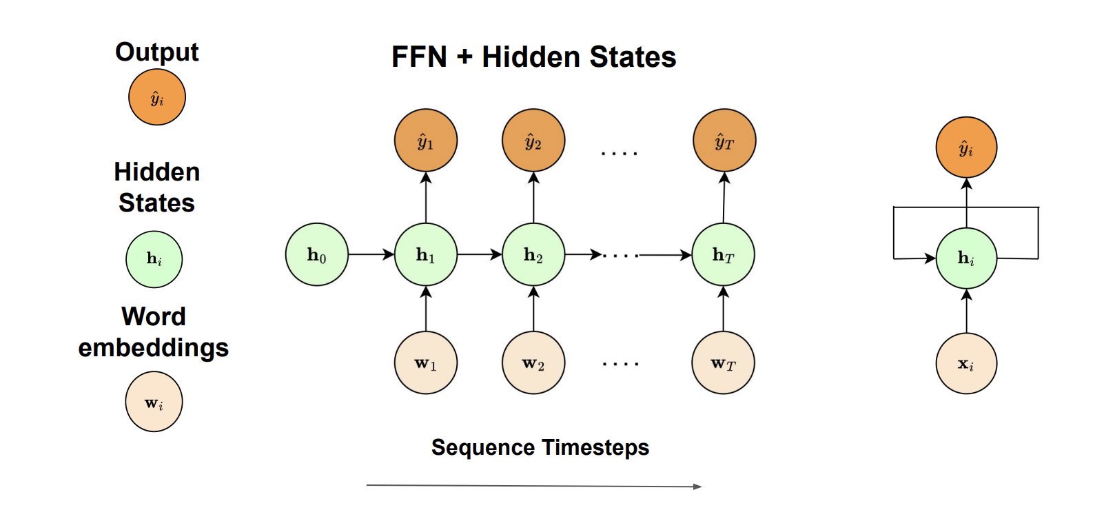
For word embedding tasks, inputs and outputs can have different lengths and features are not shared. RNNs are suited to solve these tasks by combining feedforward neural networks with hidden states to process sequential data.
At each timestep $ t $, an RNN:
* takes a word embedding $ x_t $ as input
* combines this with the previous hidden state $ h_{t-1} $
* produces an output and updates the hidden state using shared parameters
RNNs adopt parameter sharing, where the same weight matrices are used at each timestep. This significantly reduces the number of parameters and allows handling varying sequence lengths.