# Recurrent Neural Networks, LSTMs, and GRUs
## Motivation
Standard feedforward neural networks, such as MLPs, expect a fixed-size input vector and produce a fixed-size output. While this works well for tasks like image classification or regression, it poses serious limitations when working with **sequential data**—data where the order of elements matters, such as sentences, time series, or audio signals.
Consider the task of processing a sentence like "I like cats because they look cute." Each word can be mapped to a dense vector $ \mathbf{v}_i \in \mathbb{R}^d $ via a word embedding. This gives us a sequence $ \mathbf{v}_1, \mathbf{v}_2, \ldots, \mathbf{v}_T $—but how do we process this sequence *as a whole*, preserving order and capturing contextual dependencies?
Feedforward networks fall short for several reasons:
- **Variable-length inputs**: Sentences vary in length, but standard neural networks require a fixed input dimension.
- **No weight sharing across positions**: Each word position would require its own set of parameters, making the model inefficient and inflexible.
- **No memory**: The model cannot remember previous words in the sequence, so it treats each position independently.
Without memory of previous words, a model cannot distinguish between "I like cats" and "Cats like me"—both contain the same words with good embeddings, but they clearly have different meanings. To understand full sentences, we need models that can **process sequences** and **remember context**. This motivates the development of Recurrent Neural Networks (RNNs).
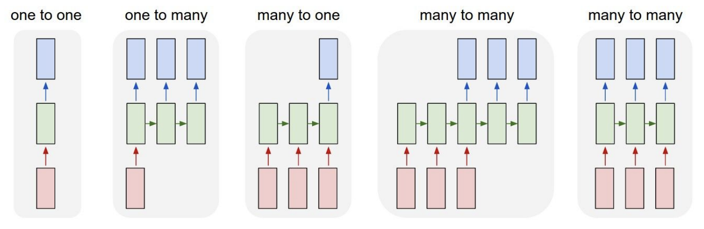 *Overview of the different input-output structures that RNNs can handle, ranging from one-to-one to many-to-many configurations.*
## Word Embeddings
Before we can feed words into any neural network, we need a way to represent them numerically. A naive approach is to use **one-hot vectors**, where each word in the vocabulary is represented as a sparse binary vector with a single 1 at the index corresponding to that word. However, one-hot vectors are high-dimensional, sparse, and fail to capture **semantic similarity**: "cat" and "dog" are just as distant as "cat" and "banana" in one-hot space.
**Word embeddings** address this by mapping each word to a **dense vector** in a continuous space. These embeddings are learned so that words appearing in similar contexts have similar vector representations. Famously, well-trained embeddings can capture semantic relationships via vector arithmetic—for example, $ \text{king} - \text{man} + \text{woman} \approx \text{queen} $.
> **Key Idea**: Words that appear in similar contexts tend to have similar meanings (the *distributional hypothesis*).
### Word2Vec
**Word2Vec** is a widely used method for learning word embeddings from a corpus. The central idea is that a word's meaning can be inferred from its surrounding context. There are two main training strategies:
#### Skip-gram
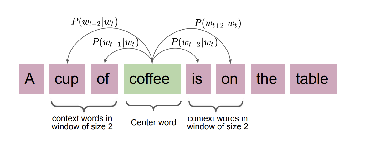
The **Skip-gram** model takes a target word and tries to predict its surrounding context words. Given a target word $ w_t $ and a context window of size $ k $, the model maximizes the probability of observing the context words $ w_c $ near $ w_t $.
The probability of a context word $ w_c $ given a target word $ w_t $ is computed using the softmax:
$$ P(w_c \mid w_t) = \frac{\exp(\mathbf{v}_{w_c}^\top \mathbf{v}_{w_t})}{\sum_{w \in V} \exp(\mathbf{v}_w^\top \mathbf{v}_{w_t})} $$
For example, with a window size of 2 around the word "coffee" in the sentence "A cup of coffee is on the table," the target is "coffee" and the context words are ["cup", "of", "is", "on"]. The model learns to predict each context word from the target.
*Overview of the different input-output structures that RNNs can handle, ranging from one-to-one to many-to-many configurations.*
## Word Embeddings
Before we can feed words into any neural network, we need a way to represent them numerically. A naive approach is to use **one-hot vectors**, where each word in the vocabulary is represented as a sparse binary vector with a single 1 at the index corresponding to that word. However, one-hot vectors are high-dimensional, sparse, and fail to capture **semantic similarity**: "cat" and "dog" are just as distant as "cat" and "banana" in one-hot space.
**Word embeddings** address this by mapping each word to a **dense vector** in a continuous space. These embeddings are learned so that words appearing in similar contexts have similar vector representations. Famously, well-trained embeddings can capture semantic relationships via vector arithmetic—for example, $ \text{king} - \text{man} + \text{woman} \approx \text{queen} $.
> **Key Idea**: Words that appear in similar contexts tend to have similar meanings (the *distributional hypothesis*).
### Word2Vec
**Word2Vec** is a widely used method for learning word embeddings from a corpus. The central idea is that a word's meaning can be inferred from its surrounding context. There are two main training strategies:
#### Skip-gram
The **Skip-gram** model takes a target word and tries to predict its surrounding context words. Given a target word $ w_t $ and a context window of size $ k $, the model maximizes the probability of observing the context words $ w_c $ near $ w_t $.
The probability of a context word $ w_c $ given a target word $ w_t $ is computed using the softmax:
$$ P(w_c \mid w_t) = \frac{\exp(\mathbf{v}_{w_c}^\top \mathbf{v}_{w_t})}{\sum_{w \in V} \exp(\mathbf{v}_w^\top \mathbf{v}_{w_t})} $$
For example, with a window size of 2 around the word "coffee" in the sentence "A cup of coffee is on the table," the target is "coffee" and the context words are ["cup", "of", "is", "on"]. The model learns to predict each context word from the target.
 *The Skip-gram model: given a target word, predict the surrounding context words. Skip-gram works well with small datasets and captures multi-context relationships.*
#### CBOW (Continuous Bag of Words)
The **Continuous Bag of Words (CBOW)** model works in the opposite direction: it predicts a target word from its surrounding context words. Given context words $ \{w_{c_1}, w_{c_2}, \ldots, w_{c_n}\} $, the model predicts the target word $ w_t $:
$$ P(w_t \mid \{w_{c_1}, \ldots, w_{c_n}\}) = \frac{\exp(\mathbf{v}_{w_t}^\top \bar{\mathbf{v}}_c)}{\sum_{w \in V} \exp(\mathbf{v}_w^\top \bar{\mathbf{v}}_c)} $$
where $ \bar{\mathbf{v}}_c = \frac{1}{n} \sum_{i=1}^{n} \mathbf{v}_{w_{c_i}} $ is the average of the context word vectors.
*The Skip-gram model: given a target word, predict the surrounding context words. Skip-gram works well with small datasets and captures multi-context relationships.*
#### CBOW (Continuous Bag of Words)
The **Continuous Bag of Words (CBOW)** model works in the opposite direction: it predicts a target word from its surrounding context words. Given context words $ \{w_{c_1}, w_{c_2}, \ldots, w_{c_n}\} $, the model predicts the target word $ w_t $:
$$ P(w_t \mid \{w_{c_1}, \ldots, w_{c_n}\}) = \frac{\exp(\mathbf{v}_{w_t}^\top \bar{\mathbf{v}}_c)}{\sum_{w \in V} \exp(\mathbf{v}_w^\top \bar{\mathbf{v}}_c)} $$
where $ \bar{\mathbf{v}}_c = \frac{1}{n} \sum_{i=1}^{n} \mathbf{v}_{w_{c_i}} $ is the average of the context word vectors.
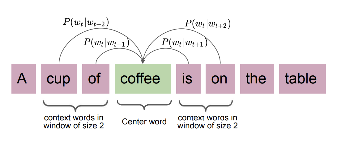 *The CBOW model: given the surrounding context words, predict the target word.*
Both models are trained by minimizing the cross-entropy loss:
$$ \mathcal{L} = -\sum_{(w_t, w_c) \in D} \log P(w_c \mid w_t) $$
### Limitations of Word2Vec
While Word2Vec produces useful embeddings, it has notable shortcomings:
- **Polysemy**: Word2Vec assigns a single static vector to each word regardless of context. The word "spring" could refer to a season or a physical object, yet it receives the same embedding in both cases.
- **Fixed window size**: The context captured is limited to a fixed window, making it difficult to learn long-range dependencies.
Contextual embedding methods (such as those used in Transformers) can address these issues by generating representations that depend on the surrounding text. Nonetheless, Word2Vec embeddings serve as effective input representations for downstream models like RNNs.
---
## RNN Architecture
### From Single Words to Sequences
To build intuition, let us start with the simplest possible setup: classifying a **single word**. Given a word represented as a vector $ \mathbf{v}_i \in \mathbb{R}^d $, we compute:
$$ \mathbf{h}_i = \sigma(\mathbf{U} \mathbf{v}_i) $$
$$ \hat{\mathbf{y}}_i = \mathbf{M} \mathbf{h}_i $$
where $ \mathbf{U} \in \mathbb{R}^{h \times d} $ maps the input to a hidden representation, $ \mathbf{M} \in \mathbb{R}^{o \times h} $ maps the hidden state to the output, and $ \sigma(\cdot) $ is a nonlinear activation function (e.g., $ \tanh $ or ReLU).
*The CBOW model: given the surrounding context words, predict the target word.*
Both models are trained by minimizing the cross-entropy loss:
$$ \mathcal{L} = -\sum_{(w_t, w_c) \in D} \log P(w_c \mid w_t) $$
### Limitations of Word2Vec
While Word2Vec produces useful embeddings, it has notable shortcomings:
- **Polysemy**: Word2Vec assigns a single static vector to each word regardless of context. The word "spring" could refer to a season or a physical object, yet it receives the same embedding in both cases.
- **Fixed window size**: The context captured is limited to a fixed window, making it difficult to learn long-range dependencies.
Contextual embedding methods (such as those used in Transformers) can address these issues by generating representations that depend on the surrounding text. Nonetheless, Word2Vec embeddings serve as effective input representations for downstream models like RNNs.
---
## RNN Architecture
### From Single Words to Sequences
To build intuition, let us start with the simplest possible setup: classifying a **single word**. Given a word represented as a vector $ \mathbf{v}_i \in \mathbb{R}^d $, we compute:
$$ \mathbf{h}_i = \sigma(\mathbf{U} \mathbf{v}_i) $$
$$ \hat{\mathbf{y}}_i = \mathbf{M} \mathbf{h}_i $$
where $ \mathbf{U} \in \mathbb{R}^{h \times d} $ maps the input to a hidden representation, $ \mathbf{M} \in \mathbb{R}^{o \times h} $ maps the hidden state to the output, and $ \sigma(\cdot) $ is a nonlinear activation function (e.g., $ \tanh $ or ReLU).
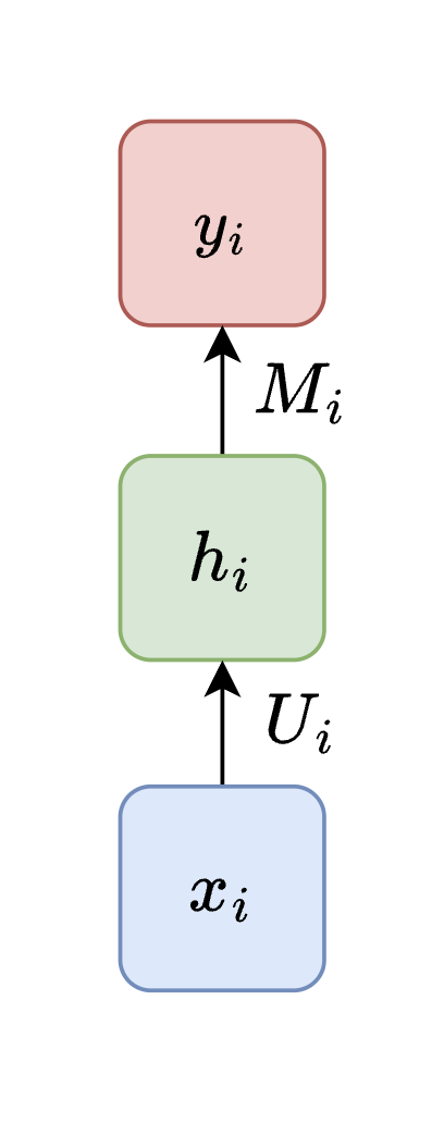 *A single-word classification model: the input word vector is transformed through a hidden layer to produce an output prediction.*
This setup processes one word at a time with no notion of sequence. To handle a sentence like "Cats look cute," we could use **separate weight matrices** at each position—$ \mathbf{U}_i, \mathbf{M}_i $ for each timestep $ i $—but this ignores the sequential nature of language and does not share any information between positions.
### Adding Recurrence
To capture dependencies between words, we introduce **connections between hidden states** across timesteps. The hidden state at each timestep now depends on both the current input $ \mathbf{v}_i $ and the previous hidden state $ \mathbf{h}_{i-1} $:
$$ \mathbf{h}_i = \sigma(\mathbf{U}_i \mathbf{v}_i + \mathbf{W}_i \mathbf{h}_{i-1}) $$
$$ \hat{\mathbf{y}}_i = \mathbf{M}_i \mathbf{h}_i $$
where $ \mathbf{W} \in \mathbb{R}^{h \times h} $ maps the previous hidden state to the current one. This gives the model memory of what came before, allowing it to incorporate **temporal context** into its predictions.
However, using separate weight matrices $ (\mathbf{U}_i, \mathbf{W}_i, \mathbf{M}_i) $ at each timestep creates two problems: (1) too many parameters for long sequences, and (2) parameters at later timesteps receive fewer training updates and may not generalize well.
### The Recurrent Neural Network
The key insight of RNNs is to **share weights across all timesteps**. We use a single set of matrices $ \mathbf{U} $, $ \mathbf{W} $, and $ \mathbf{M} $ for every position in the sequence:
$$ \mathbf{h}_t = \sigma(\mathbf{U} \mathbf{v}_t + \mathbf{W} \mathbf{h}_{t-1}) $$
$$ \hat{\mathbf{y}}_t = \mathbf{M} \mathbf{h}_t $$
*A single-word classification model: the input word vector is transformed through a hidden layer to produce an output prediction.*
This setup processes one word at a time with no notion of sequence. To handle a sentence like "Cats look cute," we could use **separate weight matrices** at each position—$ \mathbf{U}_i, \mathbf{M}_i $ for each timestep $ i $—but this ignores the sequential nature of language and does not share any information between positions.
### Adding Recurrence
To capture dependencies between words, we introduce **connections between hidden states** across timesteps. The hidden state at each timestep now depends on both the current input $ \mathbf{v}_i $ and the previous hidden state $ \mathbf{h}_{i-1} $:
$$ \mathbf{h}_i = \sigma(\mathbf{U}_i \mathbf{v}_i + \mathbf{W}_i \mathbf{h}_{i-1}) $$
$$ \hat{\mathbf{y}}_i = \mathbf{M}_i \mathbf{h}_i $$
where $ \mathbf{W} \in \mathbb{R}^{h \times h} $ maps the previous hidden state to the current one. This gives the model memory of what came before, allowing it to incorporate **temporal context** into its predictions.
However, using separate weight matrices $ (\mathbf{U}_i, \mathbf{W}_i, \mathbf{M}_i) $ at each timestep creates two problems: (1) too many parameters for long sequences, and (2) parameters at later timesteps receive fewer training updates and may not generalize well.
### The Recurrent Neural Network
The key insight of RNNs is to **share weights across all timesteps**. We use a single set of matrices $ \mathbf{U} $, $ \mathbf{W} $, and $ \mathbf{M} $ for every position in the sequence:
$$ \mathbf{h}_t = \sigma(\mathbf{U} \mathbf{v}_t + \mathbf{W} \mathbf{h}_{t-1}) $$
$$ \hat{\mathbf{y}}_t = \mathbf{M} \mathbf{h}_t $$
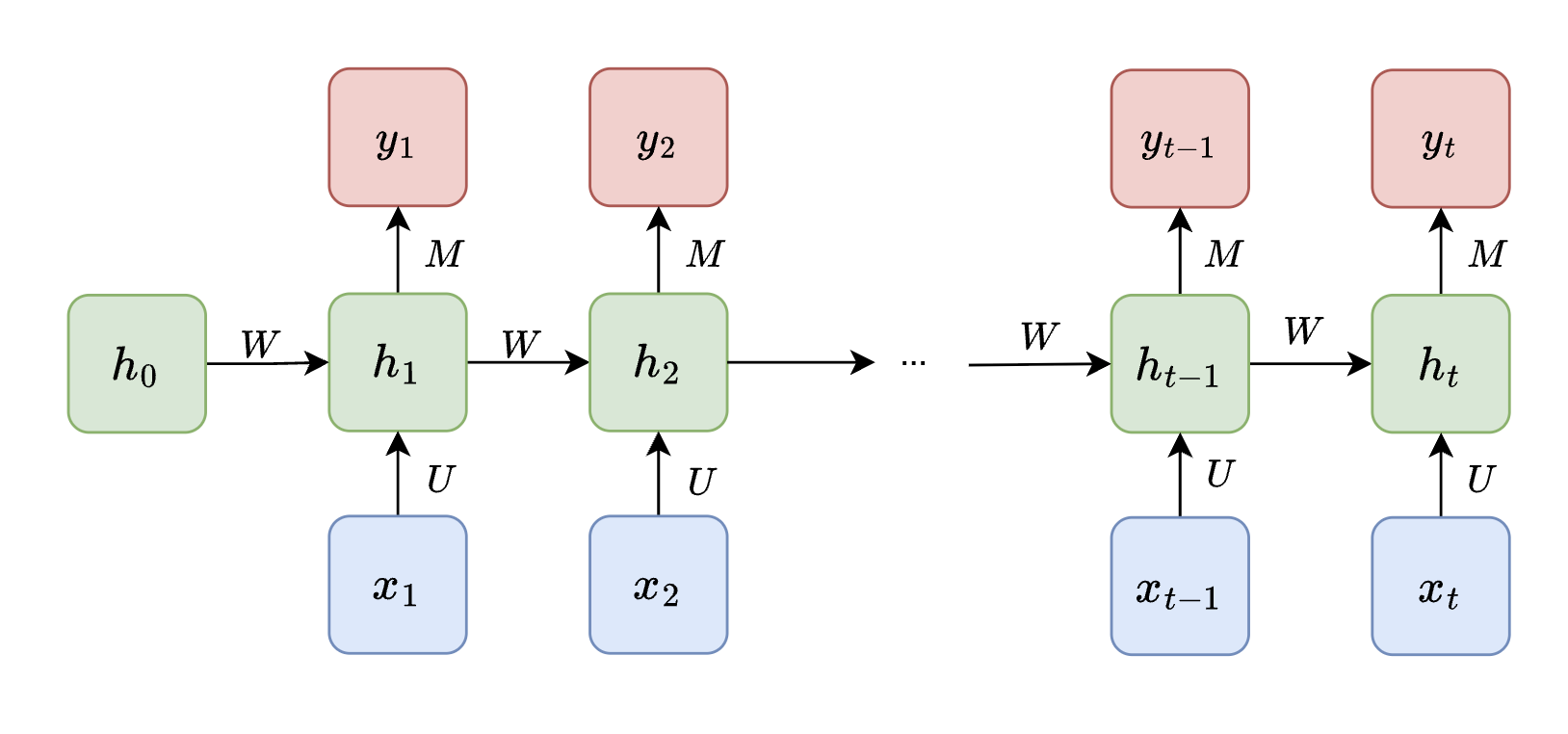 *An RNN unrolled over time. The same weight matrices $ \mathbf{U} $, $ \mathbf{W} $, and $ \mathbf{M} $ are shared across all timesteps. The initial hidden state $ \mathbf{h}_0 $ is typically initialized to zeros.*
The initial hidden state $ \mathbf{h}_0 $ is typically set to a zero vector, serving as the starting memory before any inputs are seen. Weight sharing drastically reduces the number of parameters and allows the model to generalize across sequences of varying lengths. This forms the core idea of a **Recurrent Neural Network**: a neural network that maintains and updates hidden states over time to model sequential data.
*An RNN unrolled over time. The same weight matrices $ \mathbf{U} $, $ \mathbf{W} $, and $ \mathbf{M} $ are shared across all timesteps. The initial hidden state $ \mathbf{h}_0 $ is typically initialized to zeros.*
The initial hidden state $ \mathbf{h}_0 $ is typically set to a zero vector, serving as the starting memory before any inputs are seen. Weight sharing drastically reduces the number of parameters and allows the model to generalize across sequences of varying lengths. This forms the core idea of a **Recurrent Neural Network**: a neural network that maintains and updates hidden states over time to model sequential data.
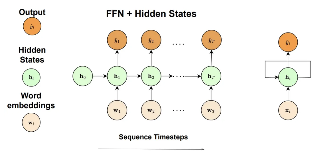 *The RNN structure showing the three main components: word embeddings as input, recurrent hidden states that carry memory across timesteps, and output predictions at each position.*
## RNN Use Cases
RNNs are remarkably flexible in their input-output configurations. Depending on the task, the same recurrent architecture can be adapted to handle different relationships between input and output sequences:
| Type | Description | Illustration | Example Use Case |
| --- | --- | --- | --- |
| One-to-One | A single input produces a single output |
*The RNN structure showing the three main components: word embeddings as input, recurrent hidden states that carry memory across timesteps, and output predictions at each position.*
## RNN Use Cases
RNNs are remarkably flexible in their input-output configurations. Depending on the task, the same recurrent architecture can be adapted to handle different relationships between input and output sequences:
| Type | Description | Illustration | Example Use Case |
| --- | --- | --- | --- |
| One-to-One | A single input produces a single output | 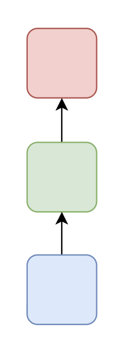 | Image classification (shown for comparison; not a typical RNN task) |
| One-to-Many | A single input leads to a sequence of outputs |
| Image classification (shown for comparison; not a typical RNN task) |
| One-to-Many | A single input leads to a sequence of outputs | 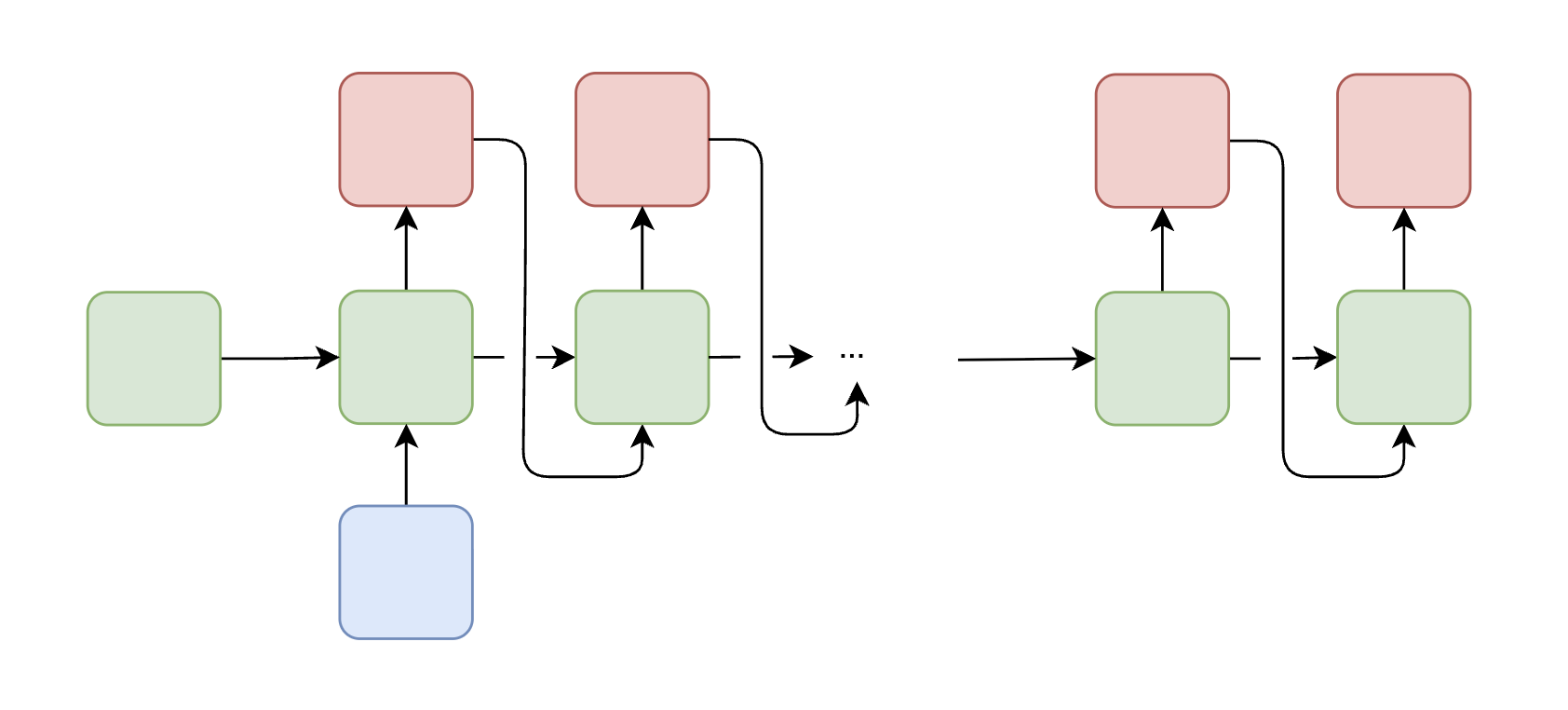 | Image captioning — given an image, generate a descriptive sentence |
| Many-to-One | A sequence of inputs produces a single output |
| Image captioning — given an image, generate a descriptive sentence |
| Many-to-One | A sequence of inputs produces a single output | 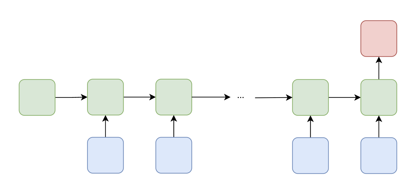 | Sentiment analysis — classify the overall sentiment of a sentence (e.g., "The product was really good!" → positive) |
| Many-to-Many (Aligned) | Each input has a corresponding output at the same position |
| Sentiment analysis — classify the overall sentiment of a sentence (e.g., "The product was really good!" → positive) |
| Many-to-Many (Aligned) | Each input has a corresponding output at the same position | 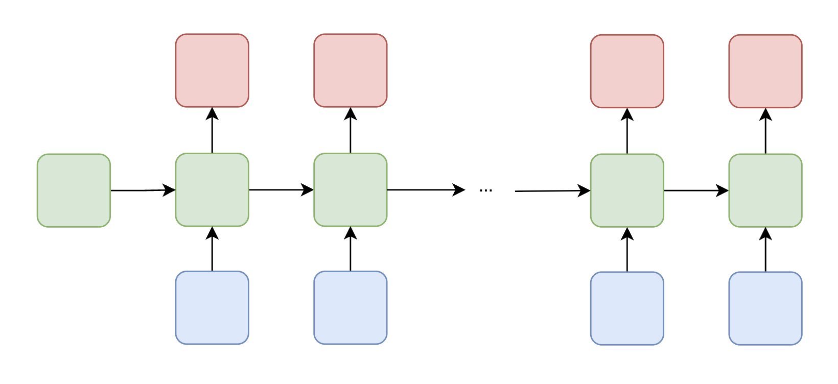 | Part-of-speech tagging — assign a grammatical label to each word in a sentence |
| Many-to-Many (Unaligned) | Input and output sequences may differ in length |
| Part-of-speech tagging — assign a grammatical label to each word in a sentence |
| Many-to-Many (Unaligned) | Input and output sequences may differ in length | 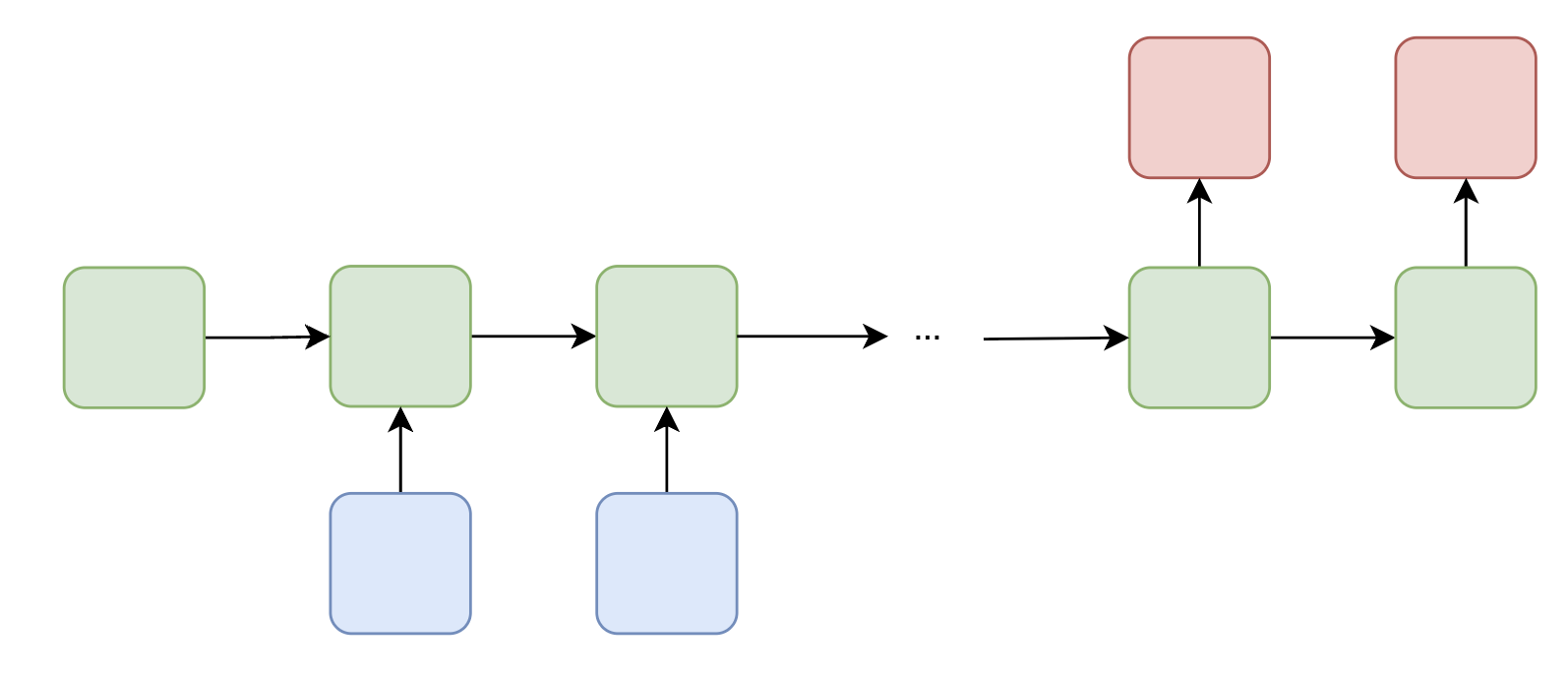 | Machine translation — an encoder RNN compresses the input into a context vector, and a decoder RNN generates the translation word by word |
These configurations illustrate the versatility of RNNs across diverse tasks in natural language processing and sequence modeling.
## Training: Backpropagation Through Time (BPTT)
Training an RNN follows the same general framework as training a feedforward network: we define a loss function, compute gradients via backpropagation, and update the weights accordingly. However, because RNNs process sequences by maintaining hidden states across timesteps, the backpropagation procedure must be adapted.
To compute gradients, we **unroll** the RNN through time, treating each timestep as a layer in a deep feedforward network with shared weights. We then apply **Backpropagation Through Time (BPTT)** to propagate error signals backward through the unrolled computation graph.
Consider a sequence of length $ T $ where the loss is computed at the final timestep:
$$ \mathcal{L}(\mathbf{y}_T, \hat{\mathbf{y}}_T) $$
The gradient of the loss with respect to the output matrix $ \mathbf{M} $ is straightforward:
$$ \frac{\partial \mathcal{L}}{\partial \mathbf{M}} = \frac{\partial \mathcal{L}}{\partial \hat{\mathbf{y}}_T} \cdot \frac{\partial \hat{\mathbf{y}}_T}{\partial \mathbf{M}} $$
However, the gradient with respect to the recurrent weight matrix $ \mathbf{W} $ is more involved, because $ \mathbf{W} $ is used at every timestep. Each timestep contributes to the total gradient. For example, with $ T = 3 $:
- From $ t = 3 $: $ \frac{\partial \mathcal{L}}{\partial \hat{\mathbf{y}}_3} \cdot \frac{\partial \hat{\mathbf{y}}_3}{\partial \mathbf{h}_3} \cdot \frac{\partial \mathbf{h}_3}{\partial \mathbf{W}} $
- From $ t = 2 $: $ \frac{\partial \mathcal{L}}{\partial \hat{\mathbf{y}}_3} \cdot \frac{\partial \hat{\mathbf{y}}_3}{\partial \mathbf{h}_3} \cdot \frac{\partial \mathbf{h}_3}{\partial \mathbf{h}_2} \cdot \frac{\partial \mathbf{h}_2}{\partial \mathbf{W}} $
- From $ t = 1 $: $ \frac{\partial \mathcal{L}}{\partial \hat{\mathbf{y}}_3} \cdot \frac{\partial \hat{\mathbf{y}}_3}{\partial \mathbf{h}_3} \cdot \frac{\partial \mathbf{h}_3}{\partial \mathbf{h}_2} \cdot \frac{\partial \mathbf{h}_2}{\partial \mathbf{h}_1} \cdot \frac{\partial \mathbf{h}_1}{\partial \mathbf{W}} $
Summing over all timesteps, the general BPTT gradient formula is:
$$ \frac{\partial \mathcal{L}}{\partial \mathbf{W}} = \sum_{t=1}^{T} \frac{\partial \mathcal{L}}{\partial \hat{\mathbf{y}}_T} \cdot \frac{\partial \hat{\mathbf{y}}_T}{\partial \mathbf{h}_T} \cdot \left( \prod_{i=t}^{T-1} \frac{\partial \mathbf{h}_{i+1}}{\partial \mathbf{h}_i} \right) \cdot \frac{\partial \mathbf{h}_t}{\partial \mathbf{W}} $$
The critical observation is the **product of Jacobians** $ \prod_{i=t}^{T-1} \frac{\partial \mathbf{h}_{i+1}}{\partial \mathbf{h}_i} $, which chains the derivatives through all intermediate hidden states. The behavior of this product determines whether training succeeds or fails for long sequences.
## Vanishing and Exploding Gradients
The product of Jacobians in the BPTT gradient is the source of one of the most fundamental challenges in training RNNs. Each factor in the product is given by:
$$ \frac{\partial \mathbf{h}_t}{\partial \mathbf{h}_{t-1}} = \text{diag}(\sigma'(\mathbf{W} \mathbf{h}_{t-1} + \mathbf{U} \mathbf{v}_t)) \cdot \mathbf{W} $$
The behavior of the full gradient depends on the spectral properties of these terms:
- **Vanishing gradients**: If $ \left\| \frac{\partial \mathbf{h}_t}{\partial \mathbf{h}_{t-1}} \right\| < 1 $ consistently, then for large $ T $, the product shrinks exponentially:
$$ \left\| \frac{\partial \mathcal{L}}{\partial \mathbf{h}_1} \right\| \to 0 $$
Early timesteps receive almost no gradient signal and fail to learn. The model effectively "forgets" information from the distant past.
- **Exploding gradients**: If $ \left\| \frac{\partial \mathbf{h}_t}{\partial \mathbf{h}_{t-1}} \right\| > 1 $ consistently, the gradient grows exponentially:
$$ \left\| \frac{\partial \mathcal{L}}{\partial \mathbf{h}_1} \right\| \to \infty $$
Parameters become unstable and training diverges. Gradient clipping can mitigate this, but it does not solve the underlying problem.
This explains why **vanilla RNNs struggle with long sequences**: the hidden states cannot reliably retain useful information across many timesteps because the gradient either vanishes or explodes during backpropagation.
### From RNNs to LSTMs: The ResNet Analogy
The vanishing gradient problem in RNNs is analogous to a well-known challenge in very deep feedforward networks. In deep networks, stacking many layers causes gradients to vanish or explode during backpropagation. The **ResNet** architecture addressed this by introducing **residual (skip) connections** that allow gradients and information to flow more directly through the network, bypassing intermediate transformations.
We can apply a similar idea to recurrent networks: what if we let information **flow across timesteps more directly**, without being constantly squashed by nonlinearities and weight multiplications? This insight leads us to the **Long Short-Term Memory (LSTM)** network.
## LSTM (Long Short-Term Memory)
The LSTM introduces a **cell state** $ \mathbf{c}_t $—a dedicated pathway that carries information across timesteps with minimal modification. Much like a ResNet's skip connection, the cell state allows gradients to flow more freely through time, preserving long-term dependencies that vanilla RNNs cannot capture.
The key properties of the LSTM cell state are:
- Information can pass forward with **minimal interference**—no repeated matrix multiplications directly on the cell state.
- Carefully designed **gates** control what information is added, removed, or revealed at each timestep.
| Machine translation — an encoder RNN compresses the input into a context vector, and a decoder RNN generates the translation word by word |
These configurations illustrate the versatility of RNNs across diverse tasks in natural language processing and sequence modeling.
## Training: Backpropagation Through Time (BPTT)
Training an RNN follows the same general framework as training a feedforward network: we define a loss function, compute gradients via backpropagation, and update the weights accordingly. However, because RNNs process sequences by maintaining hidden states across timesteps, the backpropagation procedure must be adapted.
To compute gradients, we **unroll** the RNN through time, treating each timestep as a layer in a deep feedforward network with shared weights. We then apply **Backpropagation Through Time (BPTT)** to propagate error signals backward through the unrolled computation graph.
Consider a sequence of length $ T $ where the loss is computed at the final timestep:
$$ \mathcal{L}(\mathbf{y}_T, \hat{\mathbf{y}}_T) $$
The gradient of the loss with respect to the output matrix $ \mathbf{M} $ is straightforward:
$$ \frac{\partial \mathcal{L}}{\partial \mathbf{M}} = \frac{\partial \mathcal{L}}{\partial \hat{\mathbf{y}}_T} \cdot \frac{\partial \hat{\mathbf{y}}_T}{\partial \mathbf{M}} $$
However, the gradient with respect to the recurrent weight matrix $ \mathbf{W} $ is more involved, because $ \mathbf{W} $ is used at every timestep. Each timestep contributes to the total gradient. For example, with $ T = 3 $:
- From $ t = 3 $: $ \frac{\partial \mathcal{L}}{\partial \hat{\mathbf{y}}_3} \cdot \frac{\partial \hat{\mathbf{y}}_3}{\partial \mathbf{h}_3} \cdot \frac{\partial \mathbf{h}_3}{\partial \mathbf{W}} $
- From $ t = 2 $: $ \frac{\partial \mathcal{L}}{\partial \hat{\mathbf{y}}_3} \cdot \frac{\partial \hat{\mathbf{y}}_3}{\partial \mathbf{h}_3} \cdot \frac{\partial \mathbf{h}_3}{\partial \mathbf{h}_2} \cdot \frac{\partial \mathbf{h}_2}{\partial \mathbf{W}} $
- From $ t = 1 $: $ \frac{\partial \mathcal{L}}{\partial \hat{\mathbf{y}}_3} \cdot \frac{\partial \hat{\mathbf{y}}_3}{\partial \mathbf{h}_3} \cdot \frac{\partial \mathbf{h}_3}{\partial \mathbf{h}_2} \cdot \frac{\partial \mathbf{h}_2}{\partial \mathbf{h}_1} \cdot \frac{\partial \mathbf{h}_1}{\partial \mathbf{W}} $
Summing over all timesteps, the general BPTT gradient formula is:
$$ \frac{\partial \mathcal{L}}{\partial \mathbf{W}} = \sum_{t=1}^{T} \frac{\partial \mathcal{L}}{\partial \hat{\mathbf{y}}_T} \cdot \frac{\partial \hat{\mathbf{y}}_T}{\partial \mathbf{h}_T} \cdot \left( \prod_{i=t}^{T-1} \frac{\partial \mathbf{h}_{i+1}}{\partial \mathbf{h}_i} \right) \cdot \frac{\partial \mathbf{h}_t}{\partial \mathbf{W}} $$
The critical observation is the **product of Jacobians** $ \prod_{i=t}^{T-1} \frac{\partial \mathbf{h}_{i+1}}{\partial \mathbf{h}_i} $, which chains the derivatives through all intermediate hidden states. The behavior of this product determines whether training succeeds or fails for long sequences.
## Vanishing and Exploding Gradients
The product of Jacobians in the BPTT gradient is the source of one of the most fundamental challenges in training RNNs. Each factor in the product is given by:
$$ \frac{\partial \mathbf{h}_t}{\partial \mathbf{h}_{t-1}} = \text{diag}(\sigma'(\mathbf{W} \mathbf{h}_{t-1} + \mathbf{U} \mathbf{v}_t)) \cdot \mathbf{W} $$
The behavior of the full gradient depends on the spectral properties of these terms:
- **Vanishing gradients**: If $ \left\| \frac{\partial \mathbf{h}_t}{\partial \mathbf{h}_{t-1}} \right\| < 1 $ consistently, then for large $ T $, the product shrinks exponentially:
$$ \left\| \frac{\partial \mathcal{L}}{\partial \mathbf{h}_1} \right\| \to 0 $$
Early timesteps receive almost no gradient signal and fail to learn. The model effectively "forgets" information from the distant past.
- **Exploding gradients**: If $ \left\| \frac{\partial \mathbf{h}_t}{\partial \mathbf{h}_{t-1}} \right\| > 1 $ consistently, the gradient grows exponentially:
$$ \left\| \frac{\partial \mathcal{L}}{\partial \mathbf{h}_1} \right\| \to \infty $$
Parameters become unstable and training diverges. Gradient clipping can mitigate this, but it does not solve the underlying problem.
This explains why **vanilla RNNs struggle with long sequences**: the hidden states cannot reliably retain useful information across many timesteps because the gradient either vanishes or explodes during backpropagation.
### From RNNs to LSTMs: The ResNet Analogy
The vanishing gradient problem in RNNs is analogous to a well-known challenge in very deep feedforward networks. In deep networks, stacking many layers causes gradients to vanish or explode during backpropagation. The **ResNet** architecture addressed this by introducing **residual (skip) connections** that allow gradients and information to flow more directly through the network, bypassing intermediate transformations.
We can apply a similar idea to recurrent networks: what if we let information **flow across timesteps more directly**, without being constantly squashed by nonlinearities and weight multiplications? This insight leads us to the **Long Short-Term Memory (LSTM)** network.
## LSTM (Long Short-Term Memory)
The LSTM introduces a **cell state** $ \mathbf{c}_t $—a dedicated pathway that carries information across timesteps with minimal modification. Much like a ResNet's skip connection, the cell state allows gradients to flow more freely through time, preserving long-term dependencies that vanilla RNNs cannot capture.
The key properties of the LSTM cell state are:
- Information can pass forward with **minimal interference**—no repeated matrix multiplications directly on the cell state.
- Carefully designed **gates** control what information is added, removed, or revealed at each timestep.
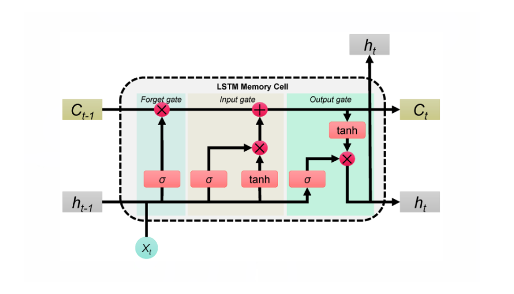 *The LSTM cell architecture showing the cell state (top horizontal line), the three gates (forget, input, output), and how they interact to update the hidden state.*
### LSTM Gates and Equations
Each LSTM cell contains three gates and a candidate update mechanism. Given the current input $ \mathbf{x}_t $, the previous hidden state $ \mathbf{h}_{t-1} $, and the previous cell state $ \mathbf{c}_{t-1} $:
**Forget Gate** — decides what information to discard from the cell state:
$$ \mathbf{f}_t = \sigma(\mathbf{W}_f [\mathbf{h}_{t-1}, \mathbf{x}_t] + \mathbf{b}_f) $$
**Input Gate** — determines what new information to write into the cell state:
$$ \mathbf{i}_t = \sigma(\mathbf{W}_i [\mathbf{h}_{t-1}, \mathbf{x}_t] + \mathbf{b}_i) $$
**Candidate Cell State** — proposes new content to potentially add:
$$ \tilde{\mathbf{c}}_t = \tanh(\mathbf{W}_c [\mathbf{h}_{t-1}, \mathbf{x}_t] + \mathbf{b}_c) $$
**Cell State Update** — combines the old cell state (filtered by the forget gate) with new information (filtered by the input gate):
$$ \mathbf{c}_t = \mathbf{f}_t \odot \mathbf{c}_{t-1} + \mathbf{i}_t \odot \tilde{\mathbf{c}}_t $$
**Output Gate** — controls what part of the cell state is exposed as the hidden state:
$$ \mathbf{o}_t = \sigma(\mathbf{W}_o [\mathbf{h}_{t-1}, \mathbf{x}_t] + \mathbf{b}_o) $$
**Hidden State Update**:
$$ \mathbf{h}_t = \mathbf{o}_t \odot \tanh(\mathbf{c}_t) $$
The cell state update equation $ \mathbf{c}_t = \mathbf{f}_t \odot \mathbf{c}_{t-1} + \mathbf{i}_t \odot \tilde{\mathbf{c}}_t $ is the critical innovation: the additive structure (rather than multiplicative) allows gradients to flow through the cell state without the compounding decay that plagues vanilla RNNs. In essence, **LSTMs solve the same problem that ResNets solved—but in time rather than depth**.
### Comparison: RNN vs. LSTM
| Feature | RNN | LSTM |
| --- | --- | --- |
| **Architecture** | Single repeating cell with tanh activation | Complex cell with input, forget, and output gates |
| **Memory** | Single hidden state (short-term only) | Cell state + hidden state (short- and long-term) |
| **Gradient Flow** | Prone to vanishing/exploding gradients | Stable gradient flow via additive cell state updates |
| **Long Sequences** | Struggles to capture long-range dependencies | Well-suited for learning long-term dependencies |
| **Computational Cost** | Lower (simpler structure, fewer parameters) | Higher (more gates, more parameters per cell) |
| **Training Stability** | Less stable, hard to converge for long sequences | More stable during training |
| **Typical Use Cases** | Simple time series, basic sequence modeling | NLP, speech recognition, video analysis, music generation |
## GRU (Gated Recurrent Unit)
While LSTMs effectively address the vanishing gradient problem, their complexity—three gates plus a separate cell state—can lead to slower training and higher computational cost. The **Gated Recurrent Unit (GRU)** provides a more efficient alternative by simplifying the LSTM architecture: it **combines the forget and input gates into a single update gate** and **merges the cell state and hidden state** into one, while retaining the ability to model long-range dependencies.
*The LSTM cell architecture showing the cell state (top horizontal line), the three gates (forget, input, output), and how they interact to update the hidden state.*
### LSTM Gates and Equations
Each LSTM cell contains three gates and a candidate update mechanism. Given the current input $ \mathbf{x}_t $, the previous hidden state $ \mathbf{h}_{t-1} $, and the previous cell state $ \mathbf{c}_{t-1} $:
**Forget Gate** — decides what information to discard from the cell state:
$$ \mathbf{f}_t = \sigma(\mathbf{W}_f [\mathbf{h}_{t-1}, \mathbf{x}_t] + \mathbf{b}_f) $$
**Input Gate** — determines what new information to write into the cell state:
$$ \mathbf{i}_t = \sigma(\mathbf{W}_i [\mathbf{h}_{t-1}, \mathbf{x}_t] + \mathbf{b}_i) $$
**Candidate Cell State** — proposes new content to potentially add:
$$ \tilde{\mathbf{c}}_t = \tanh(\mathbf{W}_c [\mathbf{h}_{t-1}, \mathbf{x}_t] + \mathbf{b}_c) $$
**Cell State Update** — combines the old cell state (filtered by the forget gate) with new information (filtered by the input gate):
$$ \mathbf{c}_t = \mathbf{f}_t \odot \mathbf{c}_{t-1} + \mathbf{i}_t \odot \tilde{\mathbf{c}}_t $$
**Output Gate** — controls what part of the cell state is exposed as the hidden state:
$$ \mathbf{o}_t = \sigma(\mathbf{W}_o [\mathbf{h}_{t-1}, \mathbf{x}_t] + \mathbf{b}_o) $$
**Hidden State Update**:
$$ \mathbf{h}_t = \mathbf{o}_t \odot \tanh(\mathbf{c}_t) $$
The cell state update equation $ \mathbf{c}_t = \mathbf{f}_t \odot \mathbf{c}_{t-1} + \mathbf{i}_t \odot \tilde{\mathbf{c}}_t $ is the critical innovation: the additive structure (rather than multiplicative) allows gradients to flow through the cell state without the compounding decay that plagues vanilla RNNs. In essence, **LSTMs solve the same problem that ResNets solved—but in time rather than depth**.
### Comparison: RNN vs. LSTM
| Feature | RNN | LSTM |
| --- | --- | --- |
| **Architecture** | Single repeating cell with tanh activation | Complex cell with input, forget, and output gates |
| **Memory** | Single hidden state (short-term only) | Cell state + hidden state (short- and long-term) |
| **Gradient Flow** | Prone to vanishing/exploding gradients | Stable gradient flow via additive cell state updates |
| **Long Sequences** | Struggles to capture long-range dependencies | Well-suited for learning long-term dependencies |
| **Computational Cost** | Lower (simpler structure, fewer parameters) | Higher (more gates, more parameters per cell) |
| **Training Stability** | Less stable, hard to converge for long sequences | More stable during training |
| **Typical Use Cases** | Simple time series, basic sequence modeling | NLP, speech recognition, video analysis, music generation |
## GRU (Gated Recurrent Unit)
While LSTMs effectively address the vanishing gradient problem, their complexity—three gates plus a separate cell state—can lead to slower training and higher computational cost. The **Gated Recurrent Unit (GRU)** provides a more efficient alternative by simplifying the LSTM architecture: it **combines the forget and input gates into a single update gate** and **merges the cell state and hidden state** into one, while retaining the ability to model long-range dependencies.
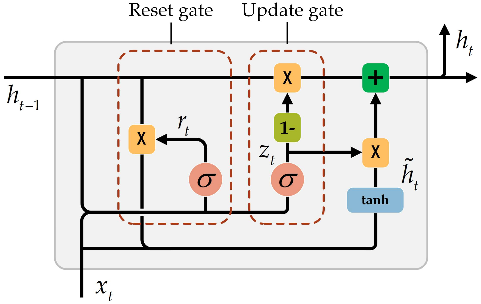 *The GRU architecture. Unlike the LSTM, the GRU maintains only a single hidden state and uses two gates (reset and update) instead of three.*
### GRU Gates and Equations
The GRU uses two gates to control information flow:
**Update Gate** — determines how much of the previous hidden state to retain:
$$ \mathbf{z}_t = \sigma(\mathbf{W}_z \mathbf{x}_t + \mathbf{U}_z \mathbf{h}_{t-1} + \mathbf{b}_z) $$
**Reset Gate** — controls how much past information to forget when computing the candidate:
$$ \mathbf{r}_t = \sigma(\mathbf{W}_r \mathbf{x}_t + \mathbf{U}_r \mathbf{h}_{t-1} + \mathbf{b}_r) $$
**Candidate Hidden State** — proposes a new hidden state, using the reset gate to potentially ignore parts of the previous state:
$$ \tilde{\mathbf{h}}_t = \tanh(\mathbf{W}_h \mathbf{x}_t + \mathbf{U}_h (\mathbf{r}_t \odot \mathbf{h}_{t-1}) + \mathbf{b}_h) $$
**Final Hidden State** — interpolates between the previous hidden state and the candidate:
$$ \mathbf{h}_t = (1 - \mathbf{z}_t) \odot \tilde{\mathbf{h}}_t + \mathbf{z}_t \odot \mathbf{h}_{t-1} $$
When $ \mathbf{z}_t \approx 1 $, the GRU copies the previous hidden state forward (preserving long-term information). When $ \mathbf{z}_t \approx 0 $, the GRU replaces it with the new candidate. This interpolation mechanism serves a similar purpose to the LSTM's cell state, but with fewer parameters and a simpler design. In practice, GRUs often achieve comparable performance to LSTMs while training faster.
## RNN Variants
Beyond the vanishing gradient problem, vanilla RNNs have additional limitations: a single-layer RNN may lack the representational capacity to capture hierarchical patterns, and processing input in only one direction ignores potentially useful future context. Two common architectural variants address these issues.
### Bidirectional RNN
In many sequence tasks, knowing both **past and future context** is beneficial. For example, the word "bank" has different meanings depending on what comes both before and after it. A standard RNN processes input only from left to right, missing future context entirely.
*The GRU architecture. Unlike the LSTM, the GRU maintains only a single hidden state and uses two gates (reset and update) instead of three.*
### GRU Gates and Equations
The GRU uses two gates to control information flow:
**Update Gate** — determines how much of the previous hidden state to retain:
$$ \mathbf{z}_t = \sigma(\mathbf{W}_z \mathbf{x}_t + \mathbf{U}_z \mathbf{h}_{t-1} + \mathbf{b}_z) $$
**Reset Gate** — controls how much past information to forget when computing the candidate:
$$ \mathbf{r}_t = \sigma(\mathbf{W}_r \mathbf{x}_t + \mathbf{U}_r \mathbf{h}_{t-1} + \mathbf{b}_r) $$
**Candidate Hidden State** — proposes a new hidden state, using the reset gate to potentially ignore parts of the previous state:
$$ \tilde{\mathbf{h}}_t = \tanh(\mathbf{W}_h \mathbf{x}_t + \mathbf{U}_h (\mathbf{r}_t \odot \mathbf{h}_{t-1}) + \mathbf{b}_h) $$
**Final Hidden State** — interpolates between the previous hidden state and the candidate:
$$ \mathbf{h}_t = (1 - \mathbf{z}_t) \odot \tilde{\mathbf{h}}_t + \mathbf{z}_t \odot \mathbf{h}_{t-1} $$
When $ \mathbf{z}_t \approx 1 $, the GRU copies the previous hidden state forward (preserving long-term information). When $ \mathbf{z}_t \approx 0 $, the GRU replaces it with the new candidate. This interpolation mechanism serves a similar purpose to the LSTM's cell state, but with fewer parameters and a simpler design. In practice, GRUs often achieve comparable performance to LSTMs while training faster.
## RNN Variants
Beyond the vanishing gradient problem, vanilla RNNs have additional limitations: a single-layer RNN may lack the representational capacity to capture hierarchical patterns, and processing input in only one direction ignores potentially useful future context. Two common architectural variants address these issues.
### Bidirectional RNN
In many sequence tasks, knowing both **past and future context** is beneficial. For example, the word "bank" has different meanings depending on what comes both before and after it. A standard RNN processes input only from left to right, missing future context entirely.
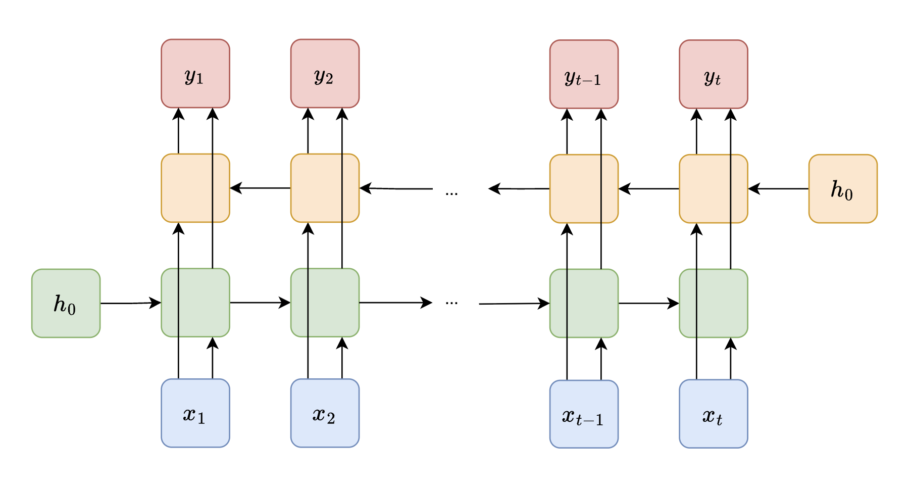 *A Bidirectional RNN runs two separate RNNs on the same input sequence: one processes from left to right (forward), and the other from right to left (backward). Their hidden states are concatenated at each timestep.*
A **Bidirectional RNN** addresses this by running two RNNs on the input:
- A **forward RNN** that processes the sequence from $ t = 1 $ to $ t = T $
- A **backward RNN** that processes from $ t = T $ to $ t = 1 $
At each timestep, the hidden states from both directions are concatenated (or otherwise combined) to form the final representation. Bidirectional RNNs are widely used in speech recognition, named entity recognition (NER), and the encoder side of machine translation systems.
### Deep RNN (Stacked RNN)
*A Bidirectional RNN runs two separate RNNs on the same input sequence: one processes from left to right (forward), and the other from right to left (backward). Their hidden states are concatenated at each timestep.*
A **Bidirectional RNN** addresses this by running two RNNs on the input:
- A **forward RNN** that processes the sequence from $ t = 1 $ to $ t = T $
- A **backward RNN** that processes from $ t = T $ to $ t = 1 $
At each timestep, the hidden states from both directions are concatenated (or otherwise combined) to form the final representation. Bidirectional RNNs are widely used in speech recognition, named entity recognition (NER), and the encoder side of machine translation systems.
### Deep RNN (Stacked RNN)
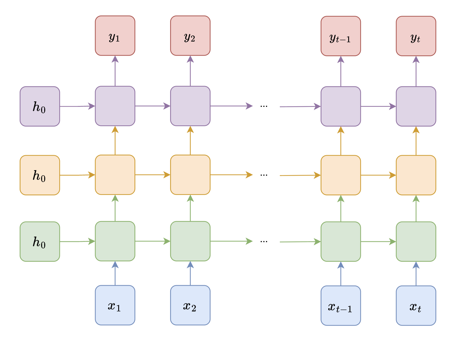 *A Deep (Stacked) RNN with multiple layers. The output of each RNN layer serves as the input to the next layer, allowing the network to learn increasingly abstract representations.*
A **Deep RNN** consists of multiple RNN layers stacked on top of each other. The output hidden states of each layer become the input to the layer above it. This depth allows:
- **Lower layers** to capture short-term, local features (e.g., word-level patterns)
- **Higher layers** to learn long-term dependencies and abstract representations (e.g., sentence-level semantics)
Stacking increases model expressiveness and has been shown to improve performance on tasks like speech recognition, machine translation, and video understanding.
## Limitations and Future Directions
Despite the advances introduced by LSTMs, GRUs, and architectural variants like bidirectional and stacked RNNs, several fundamental limitations remain:
- **Long-term dependencies**: Even with gating mechanisms, RNNs can still struggle to capture dependencies over very long sequences. The sequential nature of hidden state updates means that information must pass through every intermediate timestep to influence distant positions.
- **Sequential computation**: RNNs must process tokens one at a time in order, which prevents parallelization across the sequence dimension. This makes training significantly slower compared to architectures that can process all positions simultaneously.
- **Fixed-size hidden state**: All information about the past must be compressed into a fixed-dimensional hidden state vector, which creates an information bottleneck for long sequences.
These limitations motivated the development of **attention mechanisms** and **Transformer** architectures, which address the parallelization and long-range dependency problems by allowing direct connections between all positions in a sequence. Transformers have since become the dominant architecture for most NLP tasks and beyond.
---
__Sources__:
* [RNN/LSTM Slides](https://www.cs.cornell.edu/courses/cs4782/2025sp/slides/pdf/week5_1_slides.pdf) (CS 4/5782: Deep Learning, Spring 2025)
* [Word Embeddings Slides](https://www.cs.cornell.edu/courses/cs4782/2025sp/slides/pdf/week2_1_slides_complete.pdf) (CS 4/5782: Deep Learning, Spring 2025)
* [Understanding LSTM Networks](https://colah.github.io/posts/2015-08-Understanding-LSTMs/) (Chris Olah)
* [Illustrated Guide to LSTMs and GRUs](https://towardsdatascience.com/illustrated-guide-to-lstms-and-gru-s-a-step-by-step-explanation-44e9eb85bf21) (Towards Data Science)
* [CS231n: Recurrent Neural Networks](https://cs231n.github.io/rnn/) (Stanford)
* [Introduction to Recurrent Neural Networks](https://www.geeksforgeeks.org/introduction-to-recurrent-neural-network/) (GeeksforGeeks)
*A Deep (Stacked) RNN with multiple layers. The output of each RNN layer serves as the input to the next layer, allowing the network to learn increasingly abstract representations.*
A **Deep RNN** consists of multiple RNN layers stacked on top of each other. The output hidden states of each layer become the input to the layer above it. This depth allows:
- **Lower layers** to capture short-term, local features (e.g., word-level patterns)
- **Higher layers** to learn long-term dependencies and abstract representations (e.g., sentence-level semantics)
Stacking increases model expressiveness and has been shown to improve performance on tasks like speech recognition, machine translation, and video understanding.
## Limitations and Future Directions
Despite the advances introduced by LSTMs, GRUs, and architectural variants like bidirectional and stacked RNNs, several fundamental limitations remain:
- **Long-term dependencies**: Even with gating mechanisms, RNNs can still struggle to capture dependencies over very long sequences. The sequential nature of hidden state updates means that information must pass through every intermediate timestep to influence distant positions.
- **Sequential computation**: RNNs must process tokens one at a time in order, which prevents parallelization across the sequence dimension. This makes training significantly slower compared to architectures that can process all positions simultaneously.
- **Fixed-size hidden state**: All information about the past must be compressed into a fixed-dimensional hidden state vector, which creates an information bottleneck for long sequences.
These limitations motivated the development of **attention mechanisms** and **Transformer** architectures, which address the parallelization and long-range dependency problems by allowing direct connections between all positions in a sequence. Transformers have since become the dominant architecture for most NLP tasks and beyond.
---
__Sources__:
* [RNN/LSTM Slides](https://www.cs.cornell.edu/courses/cs4782/2025sp/slides/pdf/week5_1_slides.pdf) (CS 4/5782: Deep Learning, Spring 2025)
* [Word Embeddings Slides](https://www.cs.cornell.edu/courses/cs4782/2025sp/slides/pdf/week2_1_slides_complete.pdf) (CS 4/5782: Deep Learning, Spring 2025)
* [Understanding LSTM Networks](https://colah.github.io/posts/2015-08-Understanding-LSTMs/) (Chris Olah)
* [Illustrated Guide to LSTMs and GRUs](https://towardsdatascience.com/illustrated-guide-to-lstms-and-gru-s-a-step-by-step-explanation-44e9eb85bf21) (Towards Data Science)
* [CS231n: Recurrent Neural Networks](https://cs231n.github.io/rnn/) (Stanford)
* [Introduction to Recurrent Neural Networks](https://www.geeksforgeeks.org/introduction-to-recurrent-neural-network/) (GeeksforGeeks)