# Attention and Transformers
## Issues with LSTMs
### Issue 1: Context in Both Directions
Consider the following sentence:
As the **duck** dove underwater to catch a fish, the hunter had to **duck** quickly to avoid the low branch.
Here, the first instance of **duck** depends on the words that appear later in the sentence. However, since LSTMs are sequential, at the time of processing the first word **duck**, the LSTM cannot look ahead. As a result, an inherent limitation of LSTMs is their "single-directional" nature.
Luckily, this issue can be easily fixed through the use of Bi-directional LSTMs. Instead of having one LSTM that processes inputs only from left to right, a bidirectional LSTM uses two LSTMs in parallel—one processes inputs from left to right, and the other from right to left. Figure below shows this architecture.
> Note: Bidirectional LSTMs can be used to generate contextual word embeddings, rather than hardcoding a word to an embedding, which is what ELMo (Embeddings from Language MOdel) does!
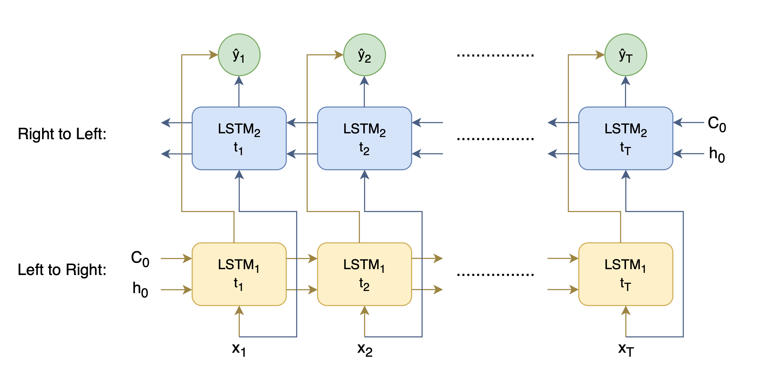 *High-level diagram of the Bi-directional LSTM architecture that produces contextual word embeddings.*
### Issue 2: The Bottleneck
In a typical encoder-decoder architecture, the entire input sequence must be compressed into the fixed-size hidden state produced by the encoder's last timestep, which is then handed off to the decoder (see figure below). This means the **final encoder output alone is responsible for summarizing all previous inputs**. Because that single vector has limited capacity, it creates a **bottleneck**: as sequence length or complexity grows, important details can be lost in compression, especially when the context is really long.
*High-level diagram of the Bi-directional LSTM architecture that produces contextual word embeddings.*
### Issue 2: The Bottleneck
In a typical encoder-decoder architecture, the entire input sequence must be compressed into the fixed-size hidden state produced by the encoder's last timestep, which is then handed off to the decoder (see figure below). This means the **final encoder output alone is responsible for summarizing all previous inputs**. Because that single vector has limited capacity, it creates a **bottleneck**: as sequence length or complexity grows, important details can be lost in compression, especially when the context is really long.
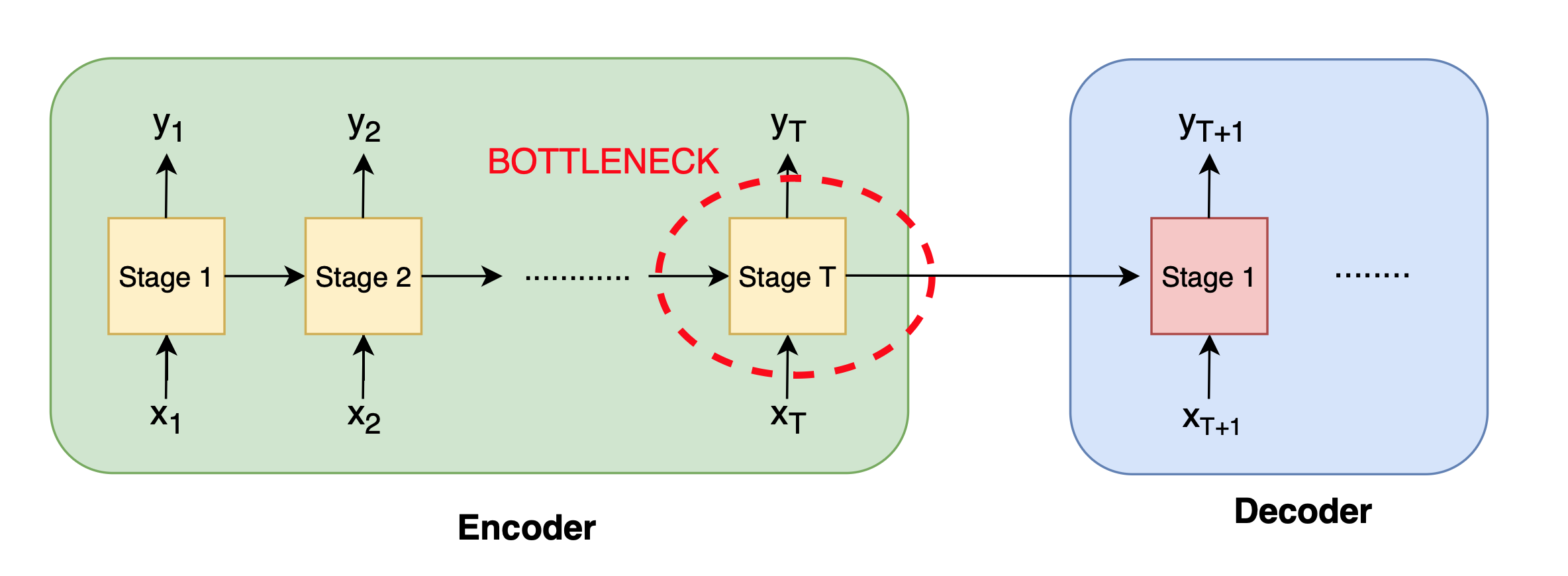 *High-level schematic of the encoder-decoder RNN architecture, highlighting the fixed-size bottleneck at the encoder's final timestep*
Rather than forcing the decoder to rely solely on the single vector $ \mathbf{h}_T $ produced by the last stage of the encoder, we make each decoder output $ \mathbf{q}_i $ attend to all encoder outputs $ \mathbf{h}_j $, obtaining a context vector $ \mathbf{x}_i $. We then concatenate $ \mathbf{x}_i $ with $ \mathbf{q}_i $, so that each decoder step has direct access to information from **all** encoder hidden states. This process is shown below mathematically and in figure below.
$$
s_i = \mathbf{q}_i \mathbf{K}^\top
$$
$$
\alpha_i = \mathrm{softmax}(s_i)
$$
$$
\mathbf{x}_i = \sum_{j=1}^{T} \alpha_{i,j} \mathbf{h}_j
$$
**Here:**
- $ \mathbf{K} = [\mathbf{h}_1, \mathbf{h}_2, \dots, \mathbf{h}_T] $: matrix of encoder hidden states (also used as keys)
- $ \mathbf{q}_i $: query vector at decoder timestep $ i $
- $ \mathbf{x}_i $: context vector at decoder step $ i $, computed as the weighted sum of encoder hidden states $ \mathbf{h}_j $
*High-level schematic of the encoder-decoder RNN architecture, highlighting the fixed-size bottleneck at the encoder's final timestep*
Rather than forcing the decoder to rely solely on the single vector $ \mathbf{h}_T $ produced by the last stage of the encoder, we make each decoder output $ \mathbf{q}_i $ attend to all encoder outputs $ \mathbf{h}_j $, obtaining a context vector $ \mathbf{x}_i $. We then concatenate $ \mathbf{x}_i $ with $ \mathbf{q}_i $, so that each decoder step has direct access to information from **all** encoder hidden states. This process is shown below mathematically and in figure below.
$$
s_i = \mathbf{q}_i \mathbf{K}^\top
$$
$$
\alpha_i = \mathrm{softmax}(s_i)
$$
$$
\mathbf{x}_i = \sum_{j=1}^{T} \alpha_{i,j} \mathbf{h}_j
$$
**Here:**
- $ \mathbf{K} = [\mathbf{h}_1, \mathbf{h}_2, \dots, \mathbf{h}_T] $: matrix of encoder hidden states (also used as keys)
- $ \mathbf{q}_i $: query vector at decoder timestep $ i $
- $ \mathbf{x}_i $: context vector at decoder step $ i $, computed as the weighted sum of encoder hidden states $ \mathbf{h}_j $
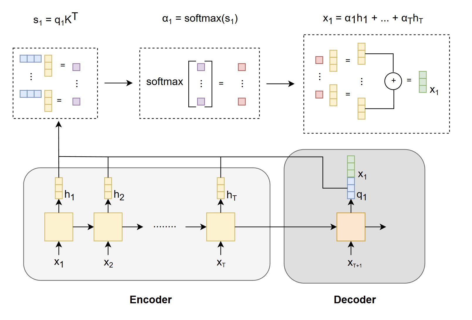 *High-level schematic of RNN with attention to solve the bottleneck issue.*
### Issue 3: Slow!
The main weakness of RNNs and LSTMs is their sequential nature: each timestep depends on the previous one, preventing parallelization. As a result, it's difficult to accelerate RNNs and LSTMs on modern hardware (with GPUs).
## Transformers
The transformer architecture introduced in *Attention is All You Need* (Vaswani et al., 2017) solves the slowness issue of RNNs and LSTMs by asking: Do we really need to pass each layer's output into the next? What if we rely solely on attention?
Since self-attention computes pairwise interactions among all tokens in parallel, it can be fully parallelized on modern hardware (e.g., GPUs), eliminating the sequential dependencies of RNNs/LSTMs.
*High-level schematic of RNN with attention to solve the bottleneck issue.*
### Issue 3: Slow!
The main weakness of RNNs and LSTMs is their sequential nature: each timestep depends on the previous one, preventing parallelization. As a result, it's difficult to accelerate RNNs and LSTMs on modern hardware (with GPUs).
## Transformers
The transformer architecture introduced in *Attention is All You Need* (Vaswani et al., 2017) solves the slowness issue of RNNs and LSTMs by asking: Do we really need to pass each layer's output into the next? What if we rely solely on attention?
Since self-attention computes pairwise interactions among all tokens in parallel, it can be fully parallelized on modern hardware (e.g., GPUs), eliminating the sequential dependencies of RNNs/LSTMs.
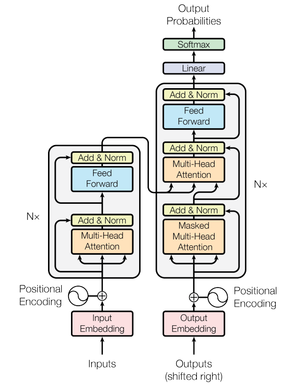 *Original transformer architecture from Attention Is All You Need.*
### Transformer Architecture: High Level
The transformer architecture proposed in the original paper uses the traditional encoder-decoder structure. At a high level, the encoder maps a sequence of symbol representations $ (\mathbf{x}_1, \ldots , \mathbf{x}_n) $ to a sequence of continuous representations $ \mathbf{z} = (\mathbf{z}_1, \ldots , \mathbf{z}_n) $. Given the continuous representations $ \mathbf{z} $, the decoder generates an output sequence $ (y_1, \ldots , y_n) $ of symbols one element at a time.
- **Preprocessing**: Before data is passed to the encoder, it is converted into embedding vectors, and positional encodings are added.
- **Encoder**: A stack of $ N $ identical layers, each with multi-head self-attention and a position-wise feed-forward network, wrapped with residual connections and layer normalization.
- **Decoder**: A stack of $ N $ identical layers with masked multi-head self-attention, cross-attention over encoder outputs, and a position-wise feed-forward network, also with residual connections and layer normalization.
The output of each sublayer is commonly written as:
$$
\text{LayerNorm}(\mathbf{x} + \text{Sublayer}(\mathbf{x}))
$$
## Transformer Components
### Components within the Transformer: Higher Level of Detail
#### Positional Embedding
Transformers process all words in a sentence **in parallel**, unlike sequential models. This greatly speeds up computation but introduces a challenge: **loss of word order information**.
Consider these two sentences:
$$
\text{"Kilian taught today's lecture, so Wei-Chiu will teach the next lecture."}\\
\text{"Wei-Chiu taught today's lecture, so Kilian will teach the next lecture."}
$$
Although both sentences use the same words, their meanings differ due to word order. Knowing who taught today's lecture depends on the position of the subject relative to the phrase "taught today's lecture", where in one case it's "Kilian", in the other, "Wei-Chiu".
To preserve positional information, we add a **positional encoding** (PE) vector to each word embedding. Each PE vector is unique to the word's position in the sentence and has the same dimensionality as the word embedding, allowing for element-wise addition.
$$
PE_{(p, 2i)} = sin(\frac{p}{10000^{\frac{2i}{d}}})
$$
$$
PE_{(p, 2i+1)} = cos(\frac{p}{10000^{\frac{2i}{d}}})
$$
where
- $ p $ is the position of the word in the sentence
- $ i $ is the dimension index
- $ d $ is the embedding size of the word vector.
Even indices use sine, odd indices use cosine. This design ensures each position has a unique encoding while allowing the model to learn relative positions.
$$
[a_1, ..., a_d] \oplus [PE_1, ..., PE_d] = [(a_1 + PE_1), ..., (a_d + PE_d)]
$$
*Original transformer architecture from Attention Is All You Need.*
### Transformer Architecture: High Level
The transformer architecture proposed in the original paper uses the traditional encoder-decoder structure. At a high level, the encoder maps a sequence of symbol representations $ (\mathbf{x}_1, \ldots , \mathbf{x}_n) $ to a sequence of continuous representations $ \mathbf{z} = (\mathbf{z}_1, \ldots , \mathbf{z}_n) $. Given the continuous representations $ \mathbf{z} $, the decoder generates an output sequence $ (y_1, \ldots , y_n) $ of symbols one element at a time.
- **Preprocessing**: Before data is passed to the encoder, it is converted into embedding vectors, and positional encodings are added.
- **Encoder**: A stack of $ N $ identical layers, each with multi-head self-attention and a position-wise feed-forward network, wrapped with residual connections and layer normalization.
- **Decoder**: A stack of $ N $ identical layers with masked multi-head self-attention, cross-attention over encoder outputs, and a position-wise feed-forward network, also with residual connections and layer normalization.
The output of each sublayer is commonly written as:
$$
\text{LayerNorm}(\mathbf{x} + \text{Sublayer}(\mathbf{x}))
$$
## Transformer Components
### Components within the Transformer: Higher Level of Detail
#### Positional Embedding
Transformers process all words in a sentence **in parallel**, unlike sequential models. This greatly speeds up computation but introduces a challenge: **loss of word order information**.
Consider these two sentences:
$$
\text{"Kilian taught today's lecture, so Wei-Chiu will teach the next lecture."}\\
\text{"Wei-Chiu taught today's lecture, so Kilian will teach the next lecture."}
$$
Although both sentences use the same words, their meanings differ due to word order. Knowing who taught today's lecture depends on the position of the subject relative to the phrase "taught today's lecture", where in one case it's "Kilian", in the other, "Wei-Chiu".
To preserve positional information, we add a **positional encoding** (PE) vector to each word embedding. Each PE vector is unique to the word's position in the sentence and has the same dimensionality as the word embedding, allowing for element-wise addition.
$$
PE_{(p, 2i)} = sin(\frac{p}{10000^{\frac{2i}{d}}})
$$
$$
PE_{(p, 2i+1)} = cos(\frac{p}{10000^{\frac{2i}{d}}})
$$
where
- $ p $ is the position of the word in the sentence
- $ i $ is the dimension index
- $ d $ is the embedding size of the word vector.
Even indices use sine, odd indices use cosine. This design ensures each position has a unique encoding while allowing the model to learn relative positions.
$$
[a_1, ..., a_d] \oplus [PE_1, ..., PE_d] = [(a_1 + PE_1), ..., (a_d + PE_d)]
$$
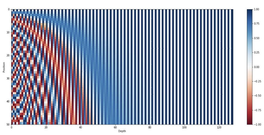 *A mapping of positional encoding vectors to colors. [source: https://www.cs.cornell.edu/courses/cs4782/2025sp/slides/pdf/week6_1.pdf]*
#### Self-Attention
You should be familiar with the equation from lecture
$$
\mathrm{Attention}(\mathbf{Q},\mathbf{K},\mathbf{V}) = \mathrm{softmax}\!\left(\frac{\mathbf{Q}\mathbf{K}^\top}{\sqrt{d_k}}\right)\mathbf{V}
$$
It is important to understand each component of the equation.
---
1. How to obtain $ \mathbf{Q}, \mathbf{K} $, and $ \mathbf{V} $:
After an input is passed through positional encoding, we obtain a feature vector $ \mathbf{x} $ for each token in the sentence. Let $ n $ be the number of tokens in the input and $ d $ be the word embedding dimension of each feature vector. Let $ \mathbf{x}_i $ be the input token at time step $ i $. The transformer creates three matrices from each feature vector $ \mathbf{x}_i \ \forall i \in [1, n] $:
- A query matrix $ \mathbf{Q} \in \mathbb{R}^{n \times d} $ where $ \mathbf{q}_i = \mathbf{W}_q \mathbf{x}_i $. This matrix represents the queries of the feature vectors or what each feature vector is looking for.
- A key matrix $ \mathbf{K} \in \mathbb{R}^{n \times d} $ where $ \mathbf{k}_i = \mathbf{W}_k \mathbf{x}_i $. This key matrix represents how each feature vector is found or what determines its compatibility.
- A value matrix $ \mathbf{V} \in \mathbb{R}^{n \times d} $ where $ \mathbf{v}_i = \mathbf{W}_v \mathbf{x}_i $. This matrix represents the true traits of each feature vector or how much each feature vector is compatible with another.
$ \mathbf{W}_q $, $ \mathbf{W}_k $, and $ \mathbf{W}_v $ are all weight matrices that are learned in training.
---
2. $ \mathbf{Q}\mathbf{K}^\top $
We compute $ \mathbf{Q}\mathbf{K}^\top $ to get an $ n \times n $ matrix of $ n^2 $ scalar values, one for each combination of pairs of words including the pair of a word with itself. The value at row $ i $ and column $ j $ can be interpreted as how much attention is the word $ i $ focusing on the word $ j $. We can also consider it the compatibility between word $ i $ and word $ j $ of a sentence. Higher values mean higher compatibility.
*A mapping of positional encoding vectors to colors. [source: https://www.cs.cornell.edu/courses/cs4782/2025sp/slides/pdf/week6_1.pdf]*
#### Self-Attention
You should be familiar with the equation from lecture
$$
\mathrm{Attention}(\mathbf{Q},\mathbf{K},\mathbf{V}) = \mathrm{softmax}\!\left(\frac{\mathbf{Q}\mathbf{K}^\top}{\sqrt{d_k}}\right)\mathbf{V}
$$
It is important to understand each component of the equation.
---
1. How to obtain $ \mathbf{Q}, \mathbf{K} $, and $ \mathbf{V} $:
After an input is passed through positional encoding, we obtain a feature vector $ \mathbf{x} $ for each token in the sentence. Let $ n $ be the number of tokens in the input and $ d $ be the word embedding dimension of each feature vector. Let $ \mathbf{x}_i $ be the input token at time step $ i $. The transformer creates three matrices from each feature vector $ \mathbf{x}_i \ \forall i \in [1, n] $:
- A query matrix $ \mathbf{Q} \in \mathbb{R}^{n \times d} $ where $ \mathbf{q}_i = \mathbf{W}_q \mathbf{x}_i $. This matrix represents the queries of the feature vectors or what each feature vector is looking for.
- A key matrix $ \mathbf{K} \in \mathbb{R}^{n \times d} $ where $ \mathbf{k}_i = \mathbf{W}_k \mathbf{x}_i $. This key matrix represents how each feature vector is found or what determines its compatibility.
- A value matrix $ \mathbf{V} \in \mathbb{R}^{n \times d} $ where $ \mathbf{v}_i = \mathbf{W}_v \mathbf{x}_i $. This matrix represents the true traits of each feature vector or how much each feature vector is compatible with another.
$ \mathbf{W}_q $, $ \mathbf{W}_k $, and $ \mathbf{W}_v $ are all weight matrices that are learned in training.
---
2. $ \mathbf{Q}\mathbf{K}^\top $
We compute $ \mathbf{Q}\mathbf{K}^\top $ to get an $ n \times n $ matrix of $ n^2 $ scalar values, one for each combination of pairs of words including the pair of a word with itself. The value at row $ i $ and column $ j $ can be interpreted as how much attention is the word $ i $ focusing on the word $ j $. We can also consider it the compatibility between word $ i $ and word $ j $ of a sentence. Higher values mean higher compatibility.
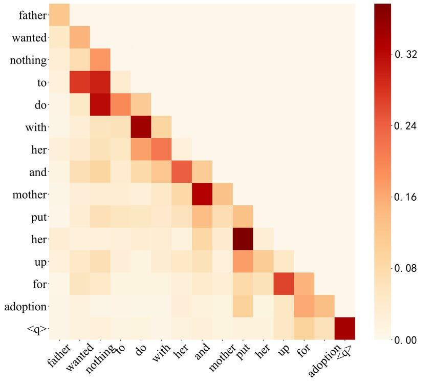 > *Attention matrix heatmap. [source: https://www.researchgate.net/figure/Heat-map-of-self-attention-on-the-decoder_fig4_365484579]*
---
3. $ \mathrm{softmax}\!\left(\frac{\mathbf{Q}\mathbf{K}^\top}{\sqrt{d_k}}\right) $
Each value in the matrix is divided by $ \sqrt{d} $ to normalize the variance of the matrix to 1. The purpose of normalizing $ \mathbf{Q}\mathbf{K}^\top $ by $ d_k $ is due to the nature of softmax. When softmax is applied, larger values become even larger, leading to a very small gradient for many weights. Normalizing the variance to 1 helps reduce the possibility of this occuring.
$$
\mathrm{softmax}(a_i) = \frac{e^{a_i}}{\sum_{j=1}^n e^{a_j} }
$$
---
4. $ \mathrm{Attention}(\mathbf{Q},\mathbf{K},\mathbf{V}) = \mathrm{softmax}\!\left(\frac{\mathbf{Q}\mathbf{K}^\top}{\sqrt{d_k}}\right)\mathbf{V} $
After obtaining the softmax scores, we multiply them with the value matrix $ \mathbf{V} $ to get an $ n \times d $ matrix. The softmax scores act as a weight which scales the $ \mathbf{V}_j $ vector based on how much attention word $ i $ focuses on each word in the sentence. Each of the $ n $ rows of the matrix represents the output word vector filled with the context of the rest of the input sequence. These output word vectors are then fed into the next sub-layer which is the feed forward neural network.
---
> *Attention matrix heatmap. [source: https://www.researchgate.net/figure/Heat-map-of-self-attention-on-the-decoder_fig4_365484579]*
---
3. $ \mathrm{softmax}\!\left(\frac{\mathbf{Q}\mathbf{K}^\top}{\sqrt{d_k}}\right) $
Each value in the matrix is divided by $ \sqrt{d} $ to normalize the variance of the matrix to 1. The purpose of normalizing $ \mathbf{Q}\mathbf{K}^\top $ by $ d_k $ is due to the nature of softmax. When softmax is applied, larger values become even larger, leading to a very small gradient for many weights. Normalizing the variance to 1 helps reduce the possibility of this occuring.
$$
\mathrm{softmax}(a_i) = \frac{e^{a_i}}{\sum_{j=1}^n e^{a_j} }
$$
---
4. $ \mathrm{Attention}(\mathbf{Q},\mathbf{K},\mathbf{V}) = \mathrm{softmax}\!\left(\frac{\mathbf{Q}\mathbf{K}^\top}{\sqrt{d_k}}\right)\mathbf{V} $
After obtaining the softmax scores, we multiply them with the value matrix $ \mathbf{V} $ to get an $ n \times d $ matrix. The softmax scores act as a weight which scales the $ \mathbf{V}_j $ vector based on how much attention word $ i $ focuses on each word in the sentence. Each of the $ n $ rows of the matrix represents the output word vector filled with the context of the rest of the input sequence. These output word vectors are then fed into the next sub-layer which is the feed forward neural network.
---
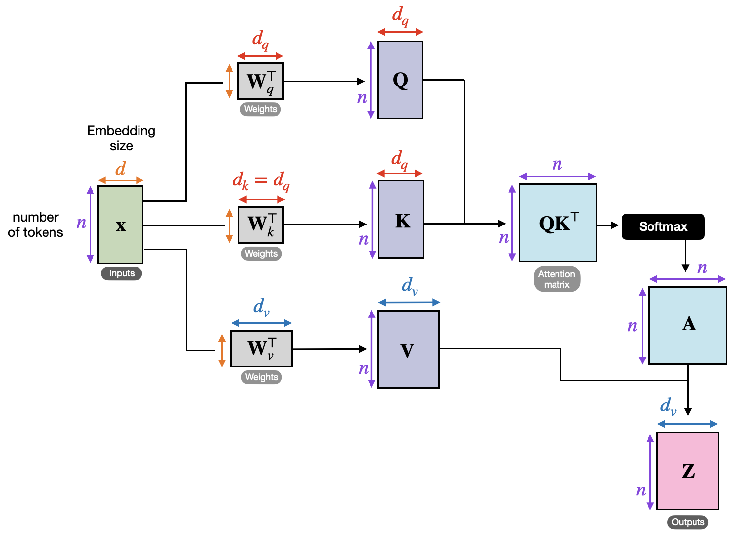 > *Self Attention Steps. [source: https://sebastianraschka.com/blog/2023/self-attention-from-scratch.html]*
In summary, self-attention takes in every feature vector and generates a context vector for each word in the sentence. This context vector is fed into the feed forward sub-layer that follows the attention sub-layer in the transformer model. A cool visualization of the self-attention process can be found [here](https://colab.research.google.com/github/tensorflow/tensor2tensor/blob/master/tensor2tensor/notebooks/hello_t2t.ipynb).
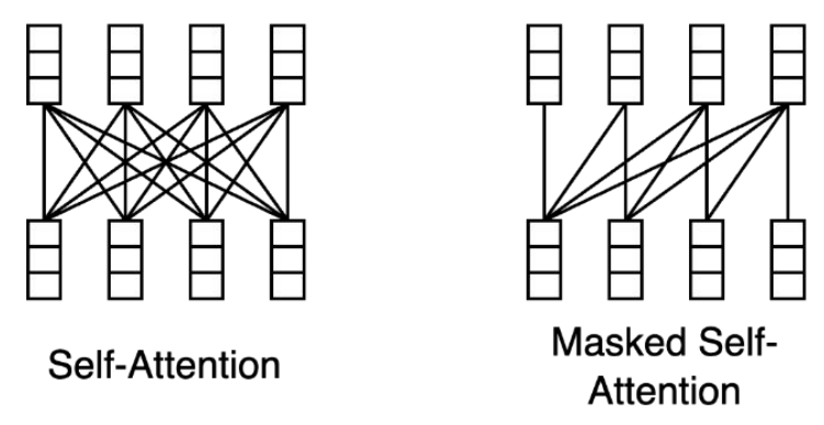
#### Masked Self-Attention
Masked self attention is a slightly different variation of self attention. In self-attention, each word can attend to any word before or after it in the sentence. In ***masked* self-attention**, however, each word can only attend to words up to the current position (i.e. words before it).
For example, consider the sentence:
> "Kilian is an awesome deep learning professor!"
In masked self-attention, at the word "awesome", the model should only have have access to the sequence "Kilian is an". The word "awesome" may attend to any of these words in this sequence, but not "deep", "learning", or "professor" which are after "awesome".
> *Self Attention Steps. [source: https://sebastianraschka.com/blog/2023/self-attention-from-scratch.html]*
In summary, self-attention takes in every feature vector and generates a context vector for each word in the sentence. This context vector is fed into the feed forward sub-layer that follows the attention sub-layer in the transformer model. A cool visualization of the self-attention process can be found [here](https://colab.research.google.com/github/tensorflow/tensor2tensor/blob/master/tensor2tensor/notebooks/hello_t2t.ipynb).
#### Masked Self-Attention
Masked self attention is a slightly different variation of self attention. In self-attention, each word can attend to any word before or after it in the sentence. In ***masked* self-attention**, however, each word can only attend to words up to the current position (i.e. words before it).
For example, consider the sentence:
> "Kilian is an awesome deep learning professor!"
In masked self-attention, at the word "awesome", the model should only have have access to the sequence "Kilian is an". The word "awesome" may attend to any of these words in this sequence, but not "deep", "learning", or "professor" which are after "awesome".
 > *Masked self Attention Matrix. [source: https://yeonwoosung.github.io/posts/what-is-gpt/]*
---
The implementation of masked self-attention mechanism is essentially the same as self-attention. The only difference is that before applying softmax, we set each value of the matrix at position $ (i, j) $ to be $ -\infty $ if $ j \gt i $. Thus, when performing softmax, these values will be zero. This ensures no word attends to word that comes after it.
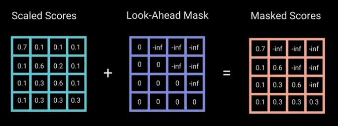
> *How the masked self attention matrix is computed. [source: https://neuron-ai.at/attention-is-all-you-need/]*
#### Multi-head Attention
Given a sentence like "Kilian and Wei-Chiu both teach CS 4782 course with great passion." we might want to focus on:
- Who ("Kilian and Wei-Chiu")
- What they do ("teach")
- How they do it ("with great passion")
Multi-head attention allows the model to focus on these different aspects simultaneously. Instead of applying attention for multiple times, it splits the attention mechanism into multiple parallel "heads", each learns to attend to a specific pattern.
> *Masked self Attention Matrix. [source: https://yeonwoosung.github.io/posts/what-is-gpt/]*
---
The implementation of masked self-attention mechanism is essentially the same as self-attention. The only difference is that before applying softmax, we set each value of the matrix at position $ (i, j) $ to be $ -\infty $ if $ j \gt i $. Thus, when performing softmax, these values will be zero. This ensures no word attends to word that comes after it.

> *How the masked self attention matrix is computed. [source: https://neuron-ai.at/attention-is-all-you-need/]*
#### Multi-head Attention
Given a sentence like "Kilian and Wei-Chiu both teach CS 4782 course with great passion." we might want to focus on:
- Who ("Kilian and Wei-Chiu")
- What they do ("teach")
- How they do it ("with great passion")
Multi-head attention allows the model to focus on these different aspects simultaneously. Instead of applying attention for multiple times, it splits the attention mechanism into multiple parallel "heads", each learns to attend to a specific pattern.
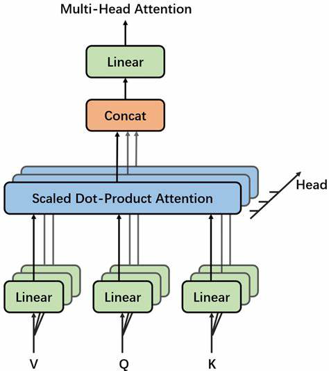 > *Multi-head attention diagram. [Source: https://www.vrogue.co/post/structure-of-multihead-attention-mechanism-download-scientific-diagram]*
How does it work?
- Given an input matrix of shape $ s \times d $, where $ s $ is the number of tokens and $ d $ is the embedding dimension.
- Compute $ \mathbf{Q}, \mathbf{K}, $ and $ \mathbf{V} $ as done in self-attention.
- Feed $ \mathbf{Q}, \mathbf{K}, $ and $ \mathbf{V} $ through a linear layer that splits them into $ h $ "heads". This operation gives us $ h $ matrices of the shape $ s \times (d/h) $. Each head operates on a different subspace of the embedding such as the examples above.
- Perform Scaled Dot-Product Attention (Per Head):
$$
\mathbf{head}_i = \mathrm{Attention}(\mathbf{W}_Q^i\mathbf{X}, \mathbf{W}_K^i\mathbf{X}, \mathbf{W}_V^i\mathbf{X})
$$
- Concatenate Heads: The $ h $ context matrices are concatenated to form an $ s \times d $ matrix.
- Perform final projection: this concatenated output is passed through another linear layer to mix information across heads.
$$
\mathrm{MultiHead}(\mathbf{X}) = \mathbf{W}_O\mathrm{Concat}(\mathbf{head}_1, \ldots, \mathbf{head}_h)
$$
The output of multi-head attention is a single matrix of the same shape as the output of self-attention. The difference is that the internal structure of multi-headed attention captures deeper and a more diverse semantic relationships. You could check out this cool visualization of multi-headed attention [Visualization of Multi-Headed Attention](https://poloclub.github.io/transformer-explainer/).
#### Cross-Attention
Cross-attention is almost identical to self-attention in process, but the inputs and execution differ:
- The key and value come from the encoder output.
- The query comes from the decoder input, which is generated one token at a time.
> *Multi-head attention diagram. [Source: https://www.vrogue.co/post/structure-of-multihead-attention-mechanism-download-scientific-diagram]*
How does it work?
- Given an input matrix of shape $ s \times d $, where $ s $ is the number of tokens and $ d $ is the embedding dimension.
- Compute $ \mathbf{Q}, \mathbf{K}, $ and $ \mathbf{V} $ as done in self-attention.
- Feed $ \mathbf{Q}, \mathbf{K}, $ and $ \mathbf{V} $ through a linear layer that splits them into $ h $ "heads". This operation gives us $ h $ matrices of the shape $ s \times (d/h) $. Each head operates on a different subspace of the embedding such as the examples above.
- Perform Scaled Dot-Product Attention (Per Head):
$$
\mathbf{head}_i = \mathrm{Attention}(\mathbf{W}_Q^i\mathbf{X}, \mathbf{W}_K^i\mathbf{X}, \mathbf{W}_V^i\mathbf{X})
$$
- Concatenate Heads: The $ h $ context matrices are concatenated to form an $ s \times d $ matrix.
- Perform final projection: this concatenated output is passed through another linear layer to mix information across heads.
$$
\mathrm{MultiHead}(\mathbf{X}) = \mathbf{W}_O\mathrm{Concat}(\mathbf{head}_1, \ldots, \mathbf{head}_h)
$$
The output of multi-head attention is a single matrix of the same shape as the output of self-attention. The difference is that the internal structure of multi-headed attention captures deeper and a more diverse semantic relationships. You could check out this cool visualization of multi-headed attention [Visualization of Multi-Headed Attention](https://poloclub.github.io/transformer-explainer/).
#### Cross-Attention
Cross-attention is almost identical to self-attention in process, but the inputs and execution differ:
- The key and value come from the encoder output.
- The query comes from the decoder input, which is generated one token at a time.
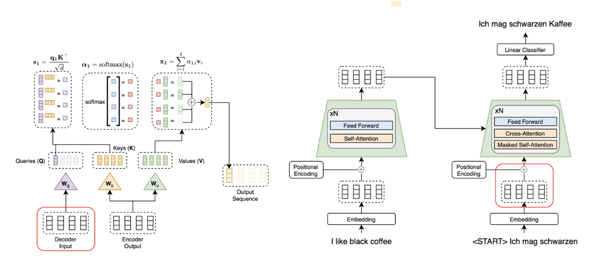 > *Cross Attention [Source: https://www.cs.cornell.edu/courses/cs4782/2025sp/slides/pdf/week6_1.pdf]*
Unlike self-attention (which uses a full matrix for parallel computation), cross-attention in the decoder is sequential. At each step:
- The current decoder token (a single word vector) is used to compute the query.
- This query attends to the encoder output (key and value matrices), producing a context vector.
- This context vector becomes part of the input for generating the next decoder token.
Since each token depends on the previous one, this process is not parallelized like in encoder attention — it proceeds one step at a time, building the context for each token sequentially.
#### Layer Norm
Layer Normalization is a technique used in neural networks to stabilize and speed up training. We use it in transformers to normalize the inputs across the features (not across the batch), especially useful since inputs vary in sequence length. Additionally, when training deep networks, internal values (activations) can become too large or too small, making training unstable. LayerNorm fixes this by scaling and shifting inputs so they have a mean of 0 and standard deviation of 1, for each input (i.e., token) individually.
Given an input vector $ \mathbf{x} = [x_1, x_2, ..., x_d] $ of dimension $ d $:
Compute the mean:
$$
\mu = \frac{1}{d}\sum_{i=1}^d x_i
$$
Then compute standard deviation:
$$
\sigma = \sqrt{\frac{1}{d}\sum_{i=1}^d (x_i-\mu)^2}
$$
Now normalize it:
$$
\hat{x}_i=\frac{x_i-\mu}{\sqrt{\sigma^2+\epsilon}}
$$
Finally, scale and shift:
$$
y_i = \gamma \hat{x}_i + \beta
$$
The layer norm is used twice per layer in the standard transformer architecture: after the self-attention + residual connection and after the feedforward network + residual connection.
---
### New Transformer Models
#### BERT
BERT (Bidirectional encoder representations from transformers) is a language model that outputs contextual word embeddings in a bidirectional context using an encoder-only transformer architecture. BERT was trained simultaneously on two tasks:
- Masked Language Model: Given a sentence, BERT masks some words in the sentence and tries to predict the original words.
- Next Sentence Prediction (NSP): Given two sentences, BERT must predict whether one sentence logically follows the other and if the second is a valid continuation of the first. In order to determine the relationship between sentences, BERT must have a fundamental sort of "understanding" of the language itself. This is what makes BERT so powerful.
BERT's fundamental understanding of the language also allows it to be fine-tuned with fewer resources and smaller datasets to address specific natural language tasks such as chatbots, question answering, or sentiment analysis.
#### T5/BART
T5 (Text-To-Text Transfer Transformer) and BART (Bidirectional and Auto-Regressive Transformer) are language models that use a pretrained encoder-decoder architecture. T5 reframes all NLP tasks: translation, summarization, classification, question answering as a single text-to-text problem, where both input and output are text strings. Both models are pretrained using a denoising objective where the model is given a corrupted version of text (e.g., with spans masked or shuffled) and learns to generate the original version.
#### GPT
GPT (Generative Pre-trained Transformer) is a stack of decoder-only Transformer blocks designed for autoregressive generation. It uses masked self-attention to ensure tokens only attend to previous positions, enabling left-to-right prediction. Each block applies layer normalization before attention and feed-forward sublayers (Pre-LN), with residual connections throughout. Positional information is added via learned embeddings, and the final output is projected to the vocabulary space for token prediction.
> *Cross Attention [Source: https://www.cs.cornell.edu/courses/cs4782/2025sp/slides/pdf/week6_1.pdf]*
Unlike self-attention (which uses a full matrix for parallel computation), cross-attention in the decoder is sequential. At each step:
- The current decoder token (a single word vector) is used to compute the query.
- This query attends to the encoder output (key and value matrices), producing a context vector.
- This context vector becomes part of the input for generating the next decoder token.
Since each token depends on the previous one, this process is not parallelized like in encoder attention — it proceeds one step at a time, building the context for each token sequentially.
#### Layer Norm
Layer Normalization is a technique used in neural networks to stabilize and speed up training. We use it in transformers to normalize the inputs across the features (not across the batch), especially useful since inputs vary in sequence length. Additionally, when training deep networks, internal values (activations) can become too large or too small, making training unstable. LayerNorm fixes this by scaling and shifting inputs so they have a mean of 0 and standard deviation of 1, for each input (i.e., token) individually.
Given an input vector $ \mathbf{x} = [x_1, x_2, ..., x_d] $ of dimension $ d $:
Compute the mean:
$$
\mu = \frac{1}{d}\sum_{i=1}^d x_i
$$
Then compute standard deviation:
$$
\sigma = \sqrt{\frac{1}{d}\sum_{i=1}^d (x_i-\mu)^2}
$$
Now normalize it:
$$
\hat{x}_i=\frac{x_i-\mu}{\sqrt{\sigma^2+\epsilon}}
$$
Finally, scale and shift:
$$
y_i = \gamma \hat{x}_i + \beta
$$
The layer norm is used twice per layer in the standard transformer architecture: after the self-attention + residual connection and after the feedforward network + residual connection.
---
### New Transformer Models
#### BERT
BERT (Bidirectional encoder representations from transformers) is a language model that outputs contextual word embeddings in a bidirectional context using an encoder-only transformer architecture. BERT was trained simultaneously on two tasks:
- Masked Language Model: Given a sentence, BERT masks some words in the sentence and tries to predict the original words.
- Next Sentence Prediction (NSP): Given two sentences, BERT must predict whether one sentence logically follows the other and if the second is a valid continuation of the first. In order to determine the relationship between sentences, BERT must have a fundamental sort of "understanding" of the language itself. This is what makes BERT so powerful.
BERT's fundamental understanding of the language also allows it to be fine-tuned with fewer resources and smaller datasets to address specific natural language tasks such as chatbots, question answering, or sentiment analysis.
#### T5/BART
T5 (Text-To-Text Transfer Transformer) and BART (Bidirectional and Auto-Regressive Transformer) are language models that use a pretrained encoder-decoder architecture. T5 reframes all NLP tasks: translation, summarization, classification, question answering as a single text-to-text problem, where both input and output are text strings. Both models are pretrained using a denoising objective where the model is given a corrupted version of text (e.g., with spans masked or shuffled) and learns to generate the original version.
#### GPT
GPT (Generative Pre-trained Transformer) is a stack of decoder-only Transformer blocks designed for autoregressive generation. It uses masked self-attention to ensure tokens only attend to previous positions, enabling left-to-right prediction. Each block applies layer normalization before attention and feed-forward sublayers (Pre-LN), with residual connections throughout. Positional information is added via learned embeddings, and the final output is projected to the vocabulary space for token prediction.
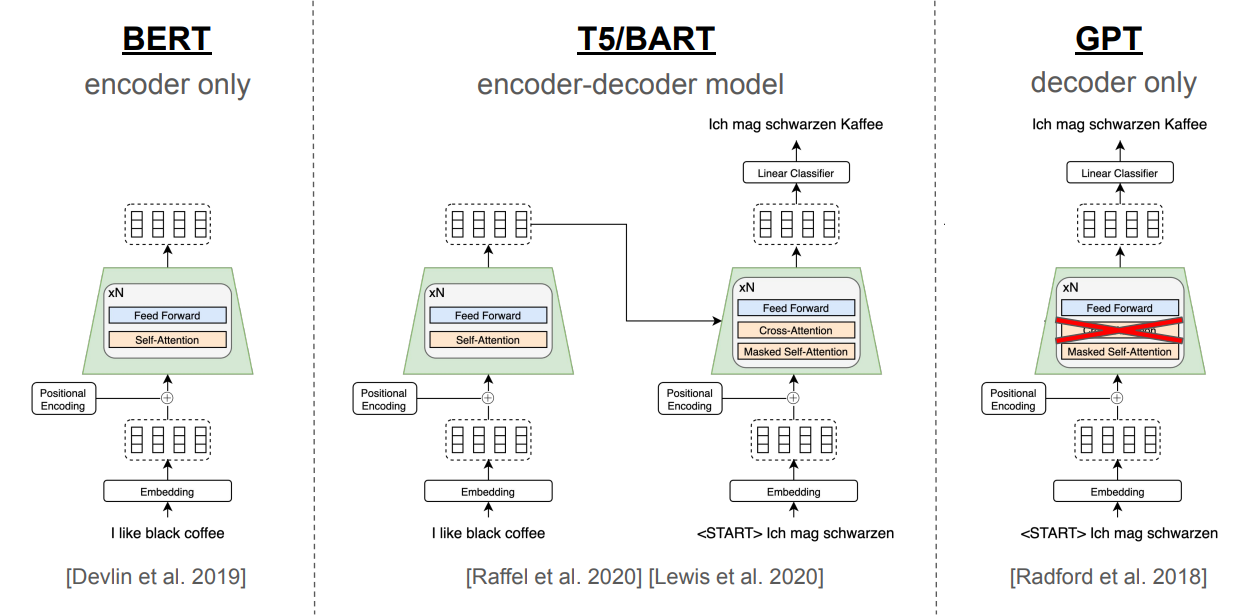 > *BERT/T5/GPT Architecture [Source: https://www.cs.cornell.edu/courses/cs4782/2025sp/slides/pdf/week6_2_slides.pdf]*
## Summary
- LSTMs still face bidirectionality limits, bottleneck compression, and sequential speed constraints which are aimed to be solved by Transformers.
- Attention in RNNs mitigates bottlenecks.
- Transformers remove recurrence, and use self-attention, masked attention, and cross-attention for scalable sequence modeling.
## References
- https://www.cs.cornell.edu/courses/cs4782/2025sp/slides/pdf/week6_1.pdf
- https://arxiv.org/pdf/1409.0473
- https://en.wikipedia.org/wiki/ELMo
- https://arxiv.org/pdf/1706.03762
- https://www.cs.cornell.edu/courses/cs4782/2025sp/slides/pdf/week6_1.pdf
- https://www.cs.cornell.edu/courses/cs4782/2025sp/slides/pdf/week6_2_slides.pdf
- https://www.researchgate.net/figure/Heat-map-of-self-attention-on-the-decoder_fig4_365484579
- https://sebastianraschka.com/blog/2023/self-attention-from-scratch.html
- https://yeonwoosung.github.io/posts/what-is-gpt/
- https://neuron-ai.at/attention-is-all-you-need/
- https://www.vrogue.co/post/structure-of-multihead-attention-mechanism-download-scientific-diagram
- https://poloclub.github.io/transformer-explainer/
> *BERT/T5/GPT Architecture [Source: https://www.cs.cornell.edu/courses/cs4782/2025sp/slides/pdf/week6_2_slides.pdf]*
## Summary
- LSTMs still face bidirectionality limits, bottleneck compression, and sequential speed constraints which are aimed to be solved by Transformers.
- Attention in RNNs mitigates bottlenecks.
- Transformers remove recurrence, and use self-attention, masked attention, and cross-attention for scalable sequence modeling.
## References
- https://www.cs.cornell.edu/courses/cs4782/2025sp/slides/pdf/week6_1.pdf
- https://arxiv.org/pdf/1409.0473
- https://en.wikipedia.org/wiki/ELMo
- https://arxiv.org/pdf/1706.03762
- https://www.cs.cornell.edu/courses/cs4782/2025sp/slides/pdf/week6_1.pdf
- https://www.cs.cornell.edu/courses/cs4782/2025sp/slides/pdf/week6_2_slides.pdf
- https://www.researchgate.net/figure/Heat-map-of-self-attention-on-the-decoder_fig4_365484579
- https://sebastianraschka.com/blog/2023/self-attention-from-scratch.html
- https://yeonwoosung.github.io/posts/what-is-gpt/
- https://neuron-ai.at/attention-is-all-you-need/
- https://www.vrogue.co/post/structure-of-multihead-attention-mechanism-download-scientific-diagram
- https://poloclub.github.io/transformer-explainer/