# Vision Pretraining (Supervised, Self-supervised)
## 1 Learning Image Representations
### 1.1 Text Representations
Recall that we can use vector spaces to represent relationships between sentences and words. One approach is representing each sentence as a bag of words, where similarity is greater when more words match:
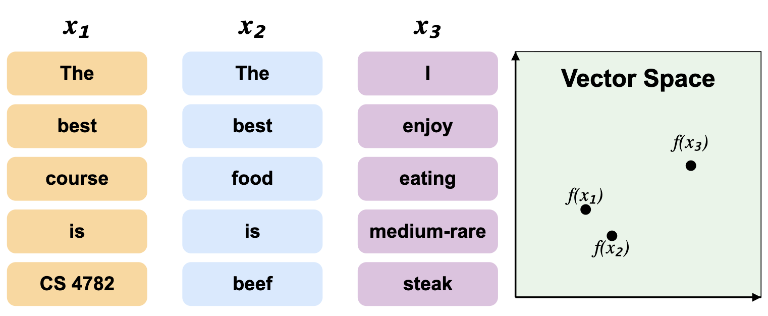
**Figure 1:** Bag of words vector space representation.
However, we see that only the trivial words are shared between $ x_1 $ and $ x_2 $, even though $ x_2 $ and $ x_3 $ are more semantically similar in terms of topic.
As we've covered before, this can be combatted by utilizing word embeddings. Here, words similar in meaning are placed close together in the vector space, and vice versa:
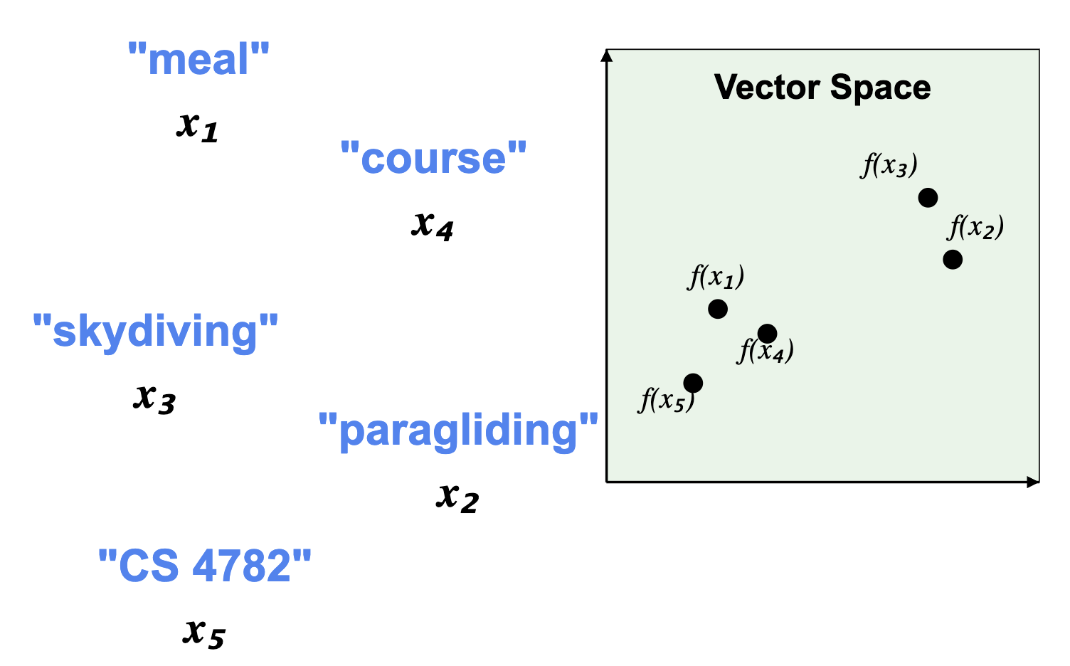
**Figure 2:** Word embeddings vector space representation.
### 1.2 Image Representations
We can start with representing images as their raw pixel values. This is analogous to the "bag-of-words" representation for text, where structurally similar images are grouped closer than semantically similar ones:
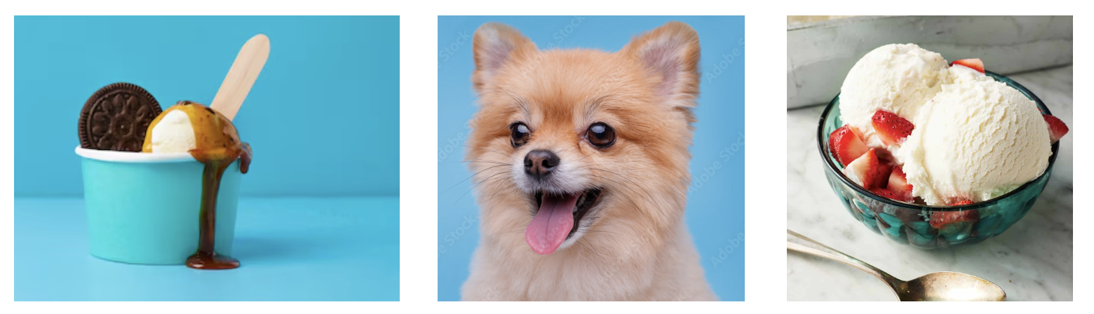
**Figure 3:** Raw pixel image representations, where structurally similar images cluster together.
Here, the blue background stands out as structurally similar, but not semantically similar. In a raw pixel representation, the first two images would be close together, but not the first and last, which both feature bowls of ice cream.
Blurry images are especially susceptible to this misclassification, as nearby pixel values are very similar.
We solve this by using classification networks to map semantically similar images to the same space. Figure 4 shows how a CNN extracts features like edges and textures before a multi-layer perceptron analyzes those weights to classify the image. These networks are much more robust to shallow variations because they focus on features rather than raw pixels.
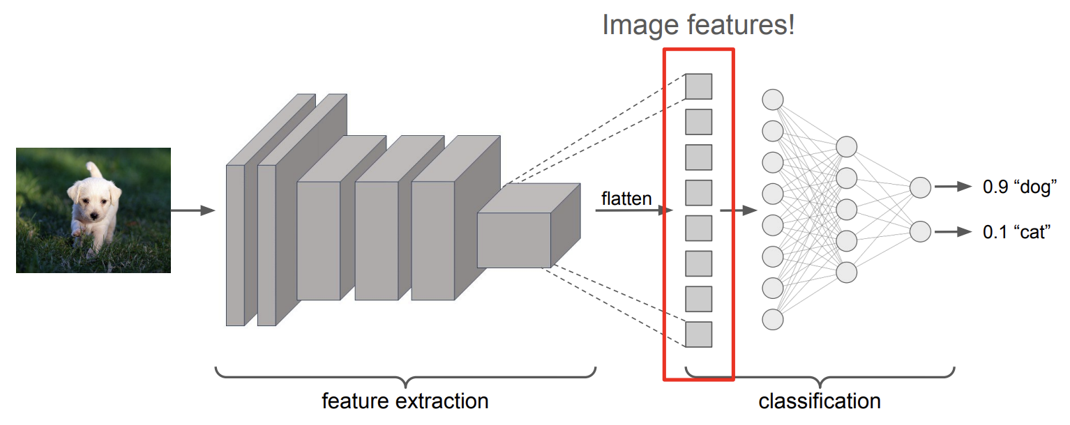
**Figure 4:** Image classification network.
## 2 Pretraining
The idea with pretraining is to first train a general purpose model on a large, diverse dataset, then customize it later for more specific tasks. As in the example for Figure 4, for supervised image classification, pre-training involves training an image classification network (e.g. trained on general images in ImageNet) and use part of it as a feature extractor, and the classification head can be fine-tuned later for other vision tasks.
Figure 5 shows that pretrained models converge much faster than models starting from scratch. The vertical-then-horizontal lines in the chart are fine-tuning performance curves that track accuracy over many iterations. The sharp vertical jumps in these curves represent points in the fine-tuning schedule where the model suddenly improves, which often happens when the learning rate is lowered to help the model settle into a better solution. A pretrained model reaches a high level of performance very early, whereas a randomly initialized model needs roughly three times as many iterations to reach the same result.
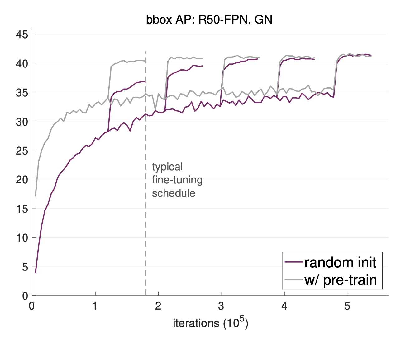
**Figure 5:** Pre-trained models converge much faster than randomly initialized ones on object detection. _(He, Kaiming, Ross Girshick, and Piotr Dollar. "Rethinking ImageNet pre-training." ICCV 2019.)_
Pretraining also enables few-shot learning, which allows us to teach a model to recognize new classes with very little labeled data because it can rely on the broad knowledge it gained during its initial training. For example, we can easily teach the model to differentiate between cats and dogs with few training data, since it already has access to the large amount of pre-training data.
### 2.1 Limitations of Supervised Pre-training
Supervised pretraining has a few major drawbacks. Sometimes the training data is not representative of what the model will see later, creating an out-of-distribution problem. Another issue is that all images must be labeled by humans, which is very expensive. This is a particular problem in specialized fields like medicine. Retinal photographs and x-rays have much higher resolution than ImageNet images and require looking for tiny tissue variations that general models might miss. Labeling these images requires expert doctors rather than general crowdsourcing, making the process even costlier. Interestingly, research shows that for some medical tasks, starting from scratch works just as well as using a pretrained model from ImageNet. This suggests that a model's performance on general images does not always predict how well it will do in a specialized domain.
## 3 Self-supervised Learning
Self-supervised learning removes the need to manually label images, which is especially valuable in specialized domains where annotated data is scarce. Self-supervised learning methods solve "pretext" tasks that produce good features for downstream tasks. For text, this may look like masking words in a sentence with the goal of predicting the masked words, as in BERT and T5.
For images, one pretext task is rotation prediction: rotate an image by one of four angles (0, 90, 180, 270 degrees) and train the model to predict which rotation was applied. To succeed at this task, the model must learn to recognize object orientation, shape, and spatial structure. These are general-purpose visual features that turn out to be useful well beyond rotation prediction itself. A ConvNet typically serves as the feature extractor for this task.
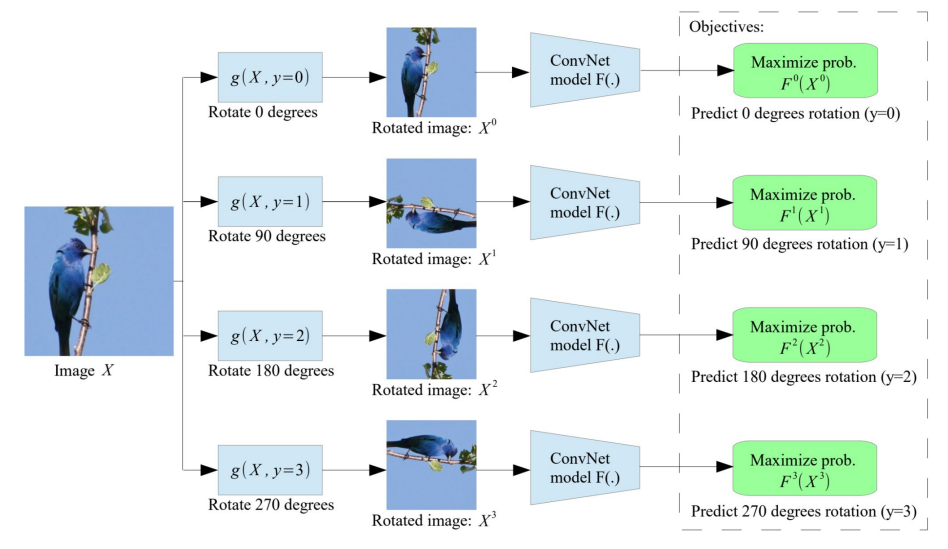
**Figure 6:** Rotation Pretext Task label generation (Gidaris, Spyros, Praveer Singh, and Nikos Komodakis. "Unsupervised Representation Learning by Predicting Image Rotations." ICLR 2018. 2018)
After pre-training, we freeze the feature extractor weights to preserve the learned representations. We then attach a shallow network on top and train only that network on a small amount of labeled data for the target task. This way, the expensive feature learning is done once during pre-training, and task-specific adaptation requires minimal labeled data.
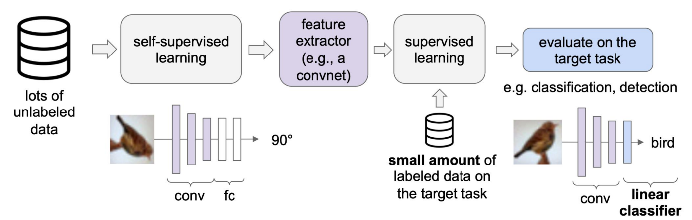
**Figure 7:** Adapting Pre-trained Network for Downstream Tasks (http://cs231n.stanford.edu/slides/2023/lecture_13.pdf)
### 3.1 Self-supervised Pre-training Accuracy
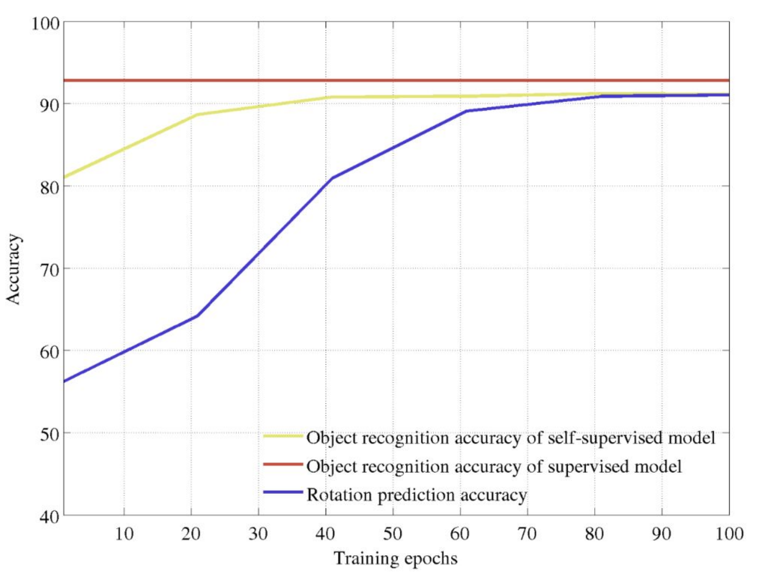
**Figure 8:** Pretraining accuracy comparison. _(Gidaris, Spyros, Praveer Singh, and Nikos Komodakis. "Unsupervised Representation Learning by Predicting Image Rotations." ICLR 2018.)_
The graph compares three metrics over training epochs: supervised object recognition accuracy (red), self-supervised object recognition accuracy (yellow), and rotation prediction accuracy (blue). The supervised model sets an upper bound at roughly 93% accuracy. As the rotation prediction pretext task improves over training, the self-supervised model's object recognition accuracy rises in tandem, eventually reaching around 91%, within a few percentage points of the fully supervised baseline. This demonstrates that learning to predict rotations, despite never seeing explicit labels, produces feature representations that transfer effectively to object recognition, nearly matching supervised performance.
## 4 Contrastive Loss
Contrastive learning is a self-supervised technique that learns representations by comparing samples against each other. Rather than predicting labels, the model learns to organize its feature space such that semantically similar inputs are mapped close together, while dissimilar inputs are pushed apart. The training signal comes entirely from the structure of the data itself.
To construct training pairs, contrastive learning relies on data augmentation. This involves applying transformations like cropping, flipping, color jittering, and rotation to a single image to produce multiple views. Since these augmented views originate from the same image, they should share the same semantic content and thus be mapped nearby in the feature space.
We define the following terms:
- **Anchor:** the original image (or one augmented view of it)
- **Positive pair:** another augmented view of the same image, which should map close to the anchor
- **Negative pair:** a view from a different image, which should map far from the anchor
The contrastive learning objective is to minimize the distance between the anchor and its positive pair, while maximizing the distance between the anchor and all negative pairs. Below, we introduce two loss functions used to achieve this.
### 4.1 Triplet Loss
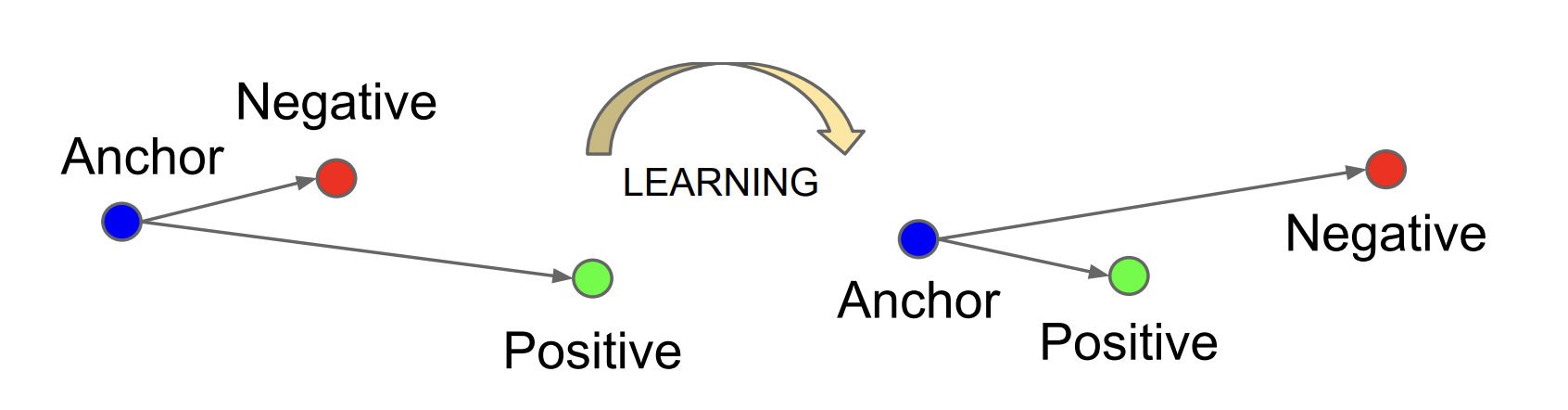
**Figure 9:** Triplet loss learns embeddings where the anchor is closer to the positive than the negative by at least a margin. _(Schroff, Florian, Dmitry Kalenichenko, and James Philbin. "FaceNet: A Unified Embedding for Face Recognition and Clustering." CVPR 2015.)_
$$l = \max(0, ||f(x_i) - f(x^+)||^2 - ||f(x_i) - f(x^-)||^2 + c)$$
- $ f $ represents our model
- $ x_i $ represents our anchor
- $ x^+ $ and $ x^- $ represent our positive and negative pairs, respectively
- $ c $ represents the margin
Important things to note:
- $ ||f(x_i) - f(x^+)||^2 $ measures how far the anchor is from the positive in embedding space. Minimizing the loss pushes this distance down.
- $ ||f(x_i) - f(x^-)||^2 $ measures how far the anchor is from the negative. Minimizing the loss pushes this distance up (since it is subtracted).
- The margin $ c $ enforces a minimum gap: the negative must be at least $ c $ farther from the anchor than the positive is. Without the margin, the model could trivially satisfy the loss by mapping everything to the same point.
- The $ \max(0, \cdot) $ function ensures the loss is zero when the margin constraint is already satisfied, so the model stops adjusting triplets that are already well-separated.
Limitations of triplet loss:
- Not differentiable at 0
- Requires explicit triplets (anchor, positive, negative), and the number of possible triplets grows as $ O(n^3) $, making triplet mining expensive
### 4.2 SimCLR
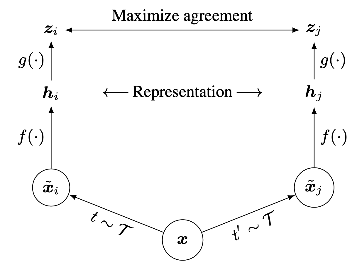
**Figure 10:** SimCLR framework: two augmented views of the same image are encoded and projected, then trained with a contrastive loss. _(Chen, Ting, et al. "A Simple Framework for Contrastive Learning of Visual Representations." ICML 2020.)_
SimCLR (Simple Framework for Contrastive Learning of Visual Representations) improves upon triplet loss by offering a more efficient approach to contrastive learning.
Key components:
- Sample two different augmentations of the same image (creates positive pairs)
- Apply a base encoder (e.g., ResNet) to each augmented view to extract image features
- Apply an MLP projection head to generate final representations that are augmentation-invariant
- The projection head is discarded after training, using only the encoder for downstream tasks
SimCLR uses a temperature-scaled cross-entropy loss. For a given anchor $ x $, the loss computes the similarity between the anchor and its positive pair relative to the similarity between the anchor and all other samples (negatives) in the batch:
$$l = -\log \left(\frac{\text{exp}(\text{sim}(x, x^+)/\tau)}{\text{exp}(\text{sim}(x, x^+)/\tau) + \text{exp}(\text{sim}(x, x^-)/\tau)}\right)$$
Here, $ \text{sim}(\cdot, \cdot) $ denotes cosine similarity between two representation vectors, and $ \tau $ is a temperature parameter that controls the sharpness of the distribution. A smaller $ \tau $ amplifies differences between similar and dissimilar pairs, while a larger $ \tau $ smooths them out. In practice, the denominator sums over all negative samples in the batch, which is why SimCLR benefits from large batch sizes.
### 4.3 Contrastive Loss Comparison
| Feature | Triplet Loss | SimCLR Loss |
| ----------------------------- | ------------------------------------------------------------------ | ------------------------------------------------------------------ |
| **Training samples** | Requires explicit triplets (anchor, positive, negative) | Uses all pairs in a batch as potential negatives |
| **Loss behavior** | Zero when margin constraint is satisfied | Never reaches exactly zero (continuous learning) |
| **Gradient behavior** | Becomes zero when well-separated | Always provides some gradient |
| **Parameter effect (small)** | Small $ c $ (0.01): Easier to satisfy; may stop learning prematurely | Small $ \tau $ (0.01): Sharp distinctions; focuses on hard negatives |
| **Parameter effect (large)** | Large $ c $ (1.0): Harder to satisfy; pushes examples further apart | Large $ \tau $ (1.0): Smoother distribution; more stable training |
| **Differentiability** | Not differentiable at the boundary point | Fully differentiable everywhere |
| **After training** | Direct use of encoder | Discard projection head; use only encoder |
| **Scaling to large datasets** | Challenging due to triplet mining needs | More efficient with batch-based negatives |
### 4.4 Momentum Contrast
SimCLR's performance depends heavily on batch size, since more samples per batch means more negatives to contrast against. This creates high memory requirements that limit scalability. Momentum Contrast (MoCo) addresses this with two key ideas:
1. **Queue-based memory bank:** Instead of drawing negatives only from the current batch, MoCo maintains a queue of encoded representations from previous batches. This provides a large, consistent pool of negatives regardless of the current batch size.
2. **Momentum encoder:** MoCo uses two encoders: a query encoder $ \theta_q $ (updated normally via backpropagation) and a key encoder $ \theta_k $ (updated slowly via exponential moving average):
$$\theta_k \leftarrow m\theta_k + (1 - m)\theta_q$$
Here, $ m $ is the momentum coefficient (typically close to 1, e.g., 0.999). The key encoder evolves slowly so that the representations stored in the queue remain consistent over time. Without this, older entries in the queue would have been encoded by a very different model, making comparisons unreliable.
The result is that MoCo decouples the number of negatives from the batch size, achieving strong contrastive learning performance with significantly lower memory requirements.
## 5 Summary
- Supervised image classification pre-training produces strong feature representations, which can efficiently transfer to other tasks
- Self-supervised learning for images include pretext tasks like rotation prediction and masked-image modeling
- Contrastive learning enforces similarity in representation space by producing image augmentations