# Vision-Language Models
## 1. Vision Transformer (ViT)
### 1.1 Introduction
As seen in previous notes, transformer architectures, originally introduced in the paper *“Attention Is All You Need”*, had a major impact on the field of NLP. However, their use in computer vision remained relatively limited until 2021, when a research team at Google published *“An Image Is Worth 16x16 Words: Transformers for Image Recognition at Scale.”* This work applied the Transformer encoder architecture to the image classification task, marking a significant step toward adapting transformers for vision applications.
The core idea of the paper is to build a Vision Transformer by leveraging the Transformer encoder architecture with minimal changes, and apply it directly to image classification tasks.
ViTs achieve competitive or superior performance when trained at scale, often with favorable scaling behavior compared to CNNs.
### 1.2 How Does ViT Work?
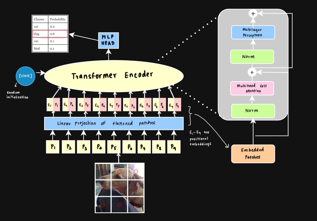
*Figure 1: Vision Transformer architecture.*
The process starts with patch embeddings. The input image is split into fixed-size patches, which are essentially small regions of the image. Each patch is then passed through a linear projection to map it into a lower-dimensional space, resulting in patch embeddings. These embeddings represent the content of their respective patches and act as the input tokens for the Transformer.
Because self-attention is permutation-invariant, learned positional embeddings are then added to the patch embeddings. Without positional embeddings, the model has no notion of spatial order. To address this, for each patch learnable positional embeddings are added to the linearly projected patch embeddings to help the model keep track of the original sequence.
The Transformer encoder is made up of several identical layers, each containing two core components: multi-head self-attention and a feedforward neural network. It takes in the patch embeddings along with their positional embeddings and processes them layer by layer, progressively refining the image representation at each stage.
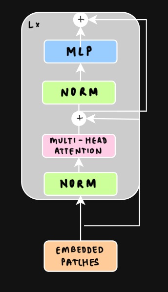
*Figure 2: Multi-head Self-Attention Module.*
Multi-head self-attention (MHSA) runs several self-attention “heads” in parallel. Each head attends over the **same set of patch tokens**, but with **different learned linear projections** for queries, keys, and values. This lets different heads learn different similarity metrics and capture different types of relationships between patches (e.g., texture vs. shape, local vs. long-range dependencies). The outputs of all heads are then concatenated and linearly combined to form the final representation.
After the self-attention step, the output is passed through a feedforward neural network (FNN aka MLP) for further transformation. This FNN consists of two linear layers with a non-linear activation function like ReLU in between (GeLU is used in the paper), allowing the model to capture more complex relationships between patches. To stabilize training, layer normalization is applied before both the self-attention and FNN blocks. Additionally, residual connections are used across each self-attention and FNN block, which helps gradients flow more smoothly during training and improves the model’s ability to learn effectively.
### 1.3 Classification Token
In addition to patch embeddings, ViT prepends a special **[CLS] token** to the input sequence.
This token acts as a **global representation of the image**.
During self-attention, the [CLS] token attends to all patch tokens and aggregates information from across the entire image. After the final transformer layer, the representation of the [CLS] token is passed through a classification head to produce the final prediction.
### 1.4 Limitations
- **Quadratic attention cost:** Self-attention scales as \(O(N^2)\) with the number of patches, making ViTs expensive for high-resolution images.
- **Weak spatial inductive bias:** Unlike CNNs, ViTs do not assume locality or translation equivariance, so spatial structure must be learned from data.
- **Lower data efficiency:** ViTs typically require large datasets or pretraining to achieve strong performance.
---
### 1.5 CNN vs. Vision Transformer (ViT)
CNNs and ViTs differ primarily in **how they process spatial structure**.
| Aspect | CNN | ViT |
|------|------|------|
| Representation | Convolutional feature maps | Sequence of image patches |
| Receptive field | Local → gradually grows with depth | Global from the first layer |
| Inductive bias | Strong (locality, translation equivariance) | Weak |
| Complexity | ~Linear with image size | Quadratic in number of patches |
| Data efficiency | Good for smaller datasets | Usually requires large-scale pretraining |
CNNs rely on strong spatial assumptions, while ViTs trade these inductive biases for **greater flexibility and global context modeling**.
#### Vision-Language Models
Another benefit of ViTs is that they produce a **sequence of visual tokens**, similar to text tokens in NLP. This representation integrates naturally with transformer-based language models, making ViTs the dominant backbone in modern vision-language systems such as CLIP and related architectures as we will see in later sections.
## 2 Swin Transformers
### 2.1 Challenges in adapting transformers to vision tasks
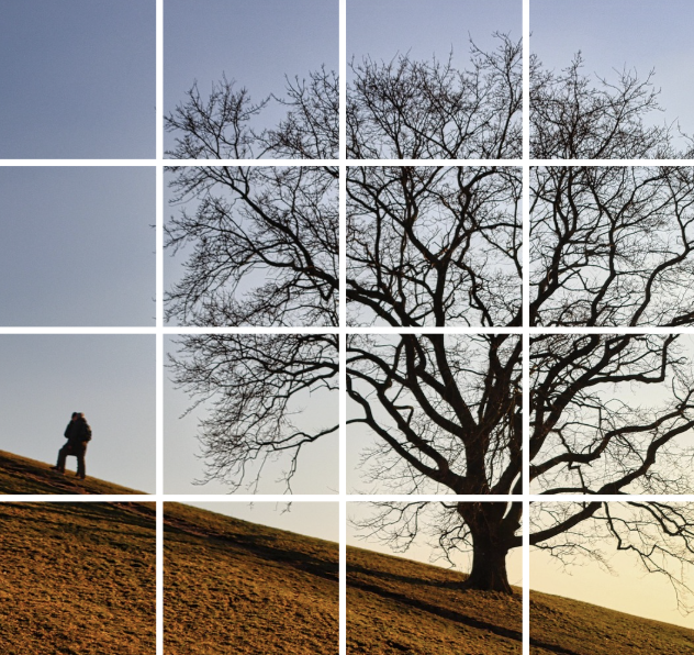
*Figure 3: Different objects have different resolutions in images. A man is in one patch, but the tree is present over multiple patches*
Vision Transformers (ViT) achieved strong results on image classification, but applying transformers to general vision tasks introduces several challenges:
- **Variation in scale of visual entities:**
In language tasks, tokens (words) are roughly uniform in size and meaning. In contrast, visual objects can vary significantly in scale (e.g., a person vs. a tree). ViT splits an image into fixed-size patches and treats each patch equally, which makes it difficult to naturally represent objects that span multiple patches or appear at different scales.
- **High-resolution images:**
Self-attention in standard transformers has **quadratic complexity with respect to the number of patches**. As image resolution increases, the number of patches grows rapidly, making global self-attention computationally expensive. This becomes especially problematic for dense prediction tasks such as **object detection** and **semantic segmentation**, which require high-resolution feature maps.
Swin Transformers address these issues through two key ideas: **hierarchical feature representations** and **shifted window attention**.
---
### 2.2 Hierarchical Architecture
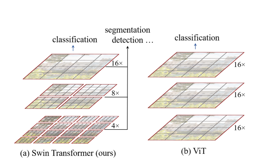
*Figure 4: Hierarchical Feature Maps. Source: [Liu et al., 2021](https://arxiv.org/pdf/2103.14030)*
Swin Transformer introduces a **hierarchical architecture**, similar to CNNs.
First, like ViT, the input image is divided into small patches that act as tokens. Note that these patches are typically smaller, so these early layers operate at **high spatial resolution**, allowing the model to capture fine visual details.
As the network becomes deeper, Swin Transformer performs **patch merging**, where neighboring patches are combined into a single token. Specifically, groups of **2 × 2 adjacent patches** are merged together.
This process works as follows:
- Four neighboring patches are grouped together.
- Their feature vectors are concatenated.
- A linear layer is applied to project the concatenated features to a new embedding dimension.
After patch merging:
- The **spatial resolution is reduced by a factor of 2** in each dimension.
- The **number of tokens decreases by 4×**.
- The **feature dimension increases**.
This has a similar effect to **downsampling in CNNs**: deeper layers operate on lower-resolution feature maps but capture larger visual patterns with a larger receptive field.
By progressively applying patch merging, Swin Transformer builds feature maps at **multiple scales**, which is important for tasks such as object detection and semantic segmentation.
---
### 2.3 Shifted Window Attention
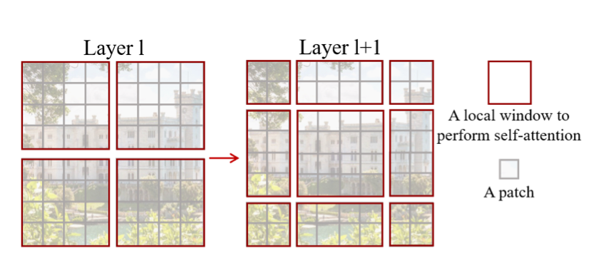
*Figure 5: Two Layer Shifted Window Attention. Source: [Liu et al., 2021](https://arxiv.org/pdf/2103.14030)*
Instead of computing self-attention across the entire image, Swin Transformer restricts attention to **local windows**.
The image is divided into small, non-overlapping windows, and self-attention is computed only among patches within each window. This approach is called **Window-based Multi-Head Self-Attention (W-MSA)**.
Since each window contains a fixed number of patches, the attention cost per window is constant. As image resolution increases, the number of windows grows linearly with image size, resulting in overall **linear complexity** with respect to the number of pixels. As a result, the total computational cost scales **linearly with image size**, making this approach much more efficient than global self-attention.
However, computing attention independently inside each window introduces a limitation: **patches in different windows cannot directly interact**.
To address this issue, Swin Transformer introduces **Shifted Window Multi-Head Self-Attention (SW-MSA)**. Instead of using the same window partition in every layer, the window grid is **shifted between consecutive layers**. This shift causes patches that were previously in different windows to be grouped together, allowing them to attend to one another.
The model alternates between two types of attention layers:
1. **W-MSA:** attention within fixed windows (Layer l in Figure 4).
2. **SW-MSA:** attention within windows that are shifted relative to the previous layer (Layer l+1 in Figure 4).
Through this alternating pattern, information can gradually propagate across the entire image while still keeping the attention computation local.
As a result, Swin Transformer achieves **linear computational complexity with respect to image size**, while still enabling interactions between distant regions of the image.
The full implementation includes additional engineering details to efficiently implement shifted window attention, but the key idea is the combination of **local window attention and shifted windows for cross-window communication**.
---
### 2.4 Performance
Swin Transformers were able to outperform the state-of-the-art ViT's at the time by ~1-2% on ImageNet-1K with significantly less computation. Additionally, they were able to use their features and achieve state-of-the-art performance on other vision tasks like object detection and semantic segmentation.
## 3 Self-Supervised Learning: DINO and MAE
Vision Transformers typically require large datasets to learn strong visual representations. However, collecting labeled data at this scale is expensive. **Self-supervised learning (SSL)** addresses this challenge by training models on **unlabeled images** using automatically generated learning objectives.
Instead of learning from human annotations, the model learns by solving a **pretext task** derived directly from the input data. Two influential approaches for training Vision Transformers with self-supervision are **DINO** and **Masked Autoencoders (MAE)**.
---
### 3.1 DINO
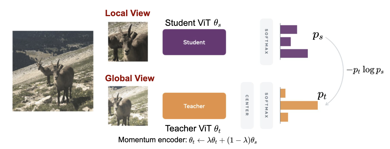
*Figure 6: DINO's self-supervised training method diagram.*
DINO (Self-**DI**stillation with **NO** labels) is a self-supervised method that trains Vision Transformers using a **teacher–student framework**. The core insight is that if a model truly understands an image, it should produce consistent representations regardless of how that image is cropped or augmented. DINO operationalizes this by training a student network to match a teacher network's output across different views of the same image.
Both the teacher and student networks share the same architecture (typically ViT). At each training step, the same image is augmented into multiple views: a few large "global" crops covering most of the image, and several small "local" crops. The student processes all views, while the teacher only sees the global crops. The student is then trained to match the teacher's output distribution, forcing it to infer global context even from a limited local view.
---
#### Important Ideas
- **Teacher–Student Training**
The student network is trained to minimize the cross-entropy between its output distribution and the teacher's output distribution on the same image. Importantly, the teacher's weights are **never updated by gradients** — this is crucial to the method.
- **Momentum Teacher (EMA)**
Instead of backpropagating into the teacher, the teacher's parameters are updated as an **exponential moving average (EMA)** of the student's weights:
$$\theta_{\text{teacher}} \leftarrow m \cdot \theta_{\text{teacher}} + (1 - m) \cdot \theta_{\text{student}}$$
where $ m $ is a momentum coefficient close to 1 (e.g., 0.996). This makes the teacher a slow-moving, stable version of the student, providing consistent training targets rather than a moving target that could destabilize learning.
- **Multi-View Learning**
Using both global and local crops creates an asymmetric training signal: the student must predict what a full view of the image looks like, having only seen a small patch. This forces the model to build semantically meaningful representations that capture global image structure.
- **Collapse Prevention**
Without safeguards, the model can "collapse" when the network learns to output the same constant representation for every image, trivially satisfying the loss. DINO prevents this with two techniques:
- **Centering:** A running mean of the teacher's outputs is subtracted from the teacher's predictions, preventing any single output dimension from dominating.
- **Sharpening:** A low temperature is applied to the teacher's softmax, producing peaked (confident) output distributions that are harder to trivially match.
---
#### What DINO Learns
DINO-trained ViTs learn surprisingly strong semantic representations without any labels. An interesting demonstration is visualizing the self-attention of the [CLS] token in the final layer: the model naturally segments foreground objects from background, highlighting **object boundaries and semantic regions** that align closely with human perception (see Figure 7).
These learned features transfer well to downstream tasks including classification, segmentation, and image retrieval — often matching or exceeding supervised baselines.
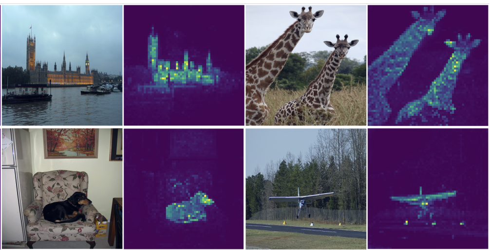
*Figure 7: Self-attention maps of the [CLS] token on the last transformer layer. No labels or supervision were used — the model learns to localize objects purely from self-distillation. (Caron et al., 2021)*
---
### 3.2 Masked Autoencoders (MAE)
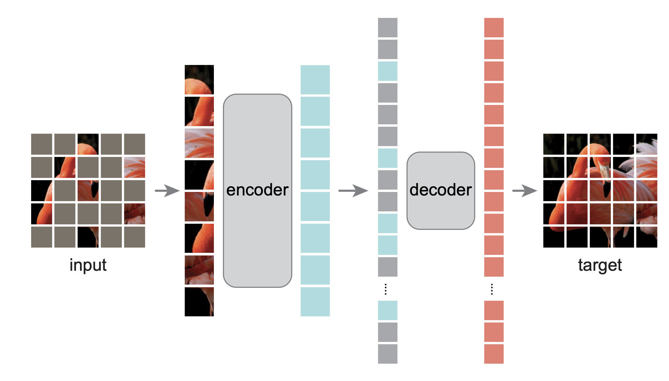
*Figure 8: MAE Architecture.*
Masked Autoencoders (MAE) take a different approach inspired by masked language modeling in NLP.
Instead of predicting labels, the model learns by **reconstructing missing parts of the input image**.
The training process works as follows:
1. **Masking:**
A large portion of image patches (often around 75%) is randomly removed.
2. **Encoder:**
A Vision Transformer encoder processes only the **visible patches**, producing a latent representation.
3. **Decoder:**
A lightweight decoder reconstructs the missing patches from the latent representation.
4. **Reconstruction Loss:**
The model is trained to minimize the difference between the reconstructed and original image patches.
By learning to reconstruct missing regions, the model captures the **global structure and semantics of images** without requiring labeled data. After pretraining, the encoder can be fine-tuned for downstream tasks such as classification, detection, and segmentation.
---
### 3.3 Summary
Both methods enable Vision Transformers to learn strong visual representations **without labeled data**, but they differ in their learning objective:
| Method | Core Idea |
|------|------|
| **DINO** | Learn invariant representations by matching predictions between teacher and student networks |
| **MAE** | Learn image structure by reconstructing masked image patches |
## 4 CLIP
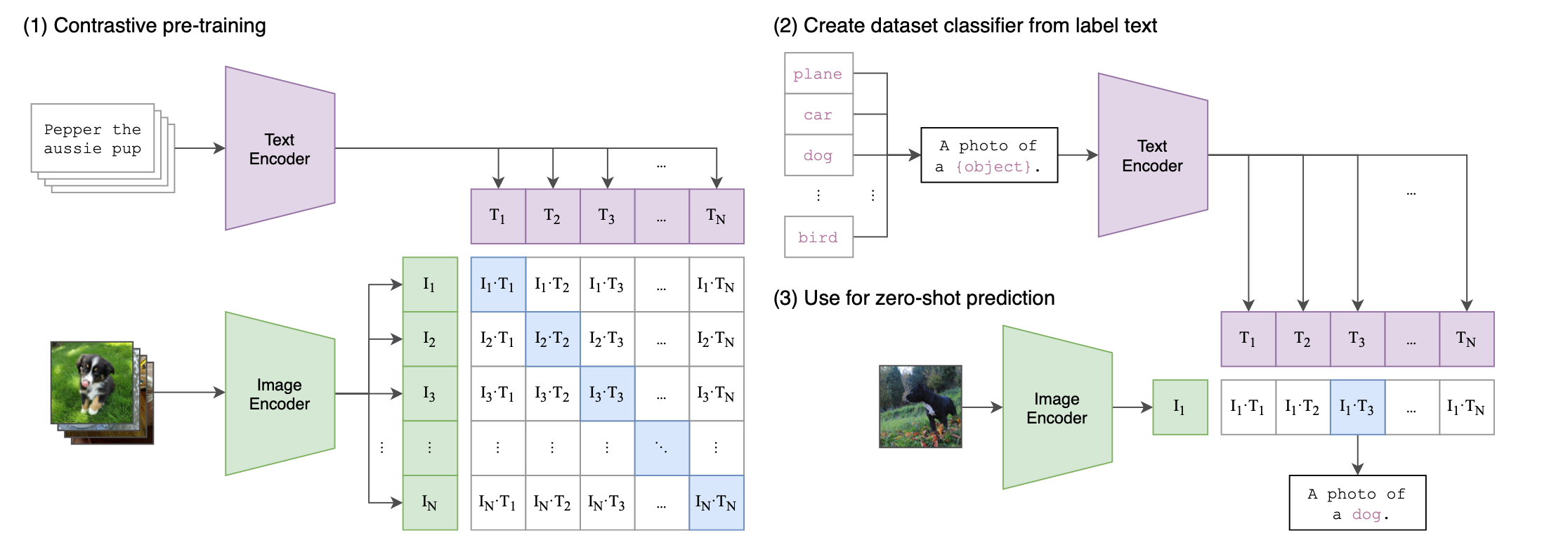
*Figure 9: CLIP Architecture.*
CLIP learns **joint representations of images and text** by training on large collections of image–caption pairs.
**Key idea:**
Learn a shared embedding space where matching image–text pairs are close together and mismatched pairs are far apart.
---
### 4.1 Model Architecture
CLIP consists of two encoders trained jointly. The **text encoder** is typically a transformer that encodes a caption into a fixed-length vector representation.
Example: `"Pepper the Aussie pup" → text embedding`
The **image encoder** can be either a ViT or a CNN and encodes an image into a vector representation.
Example: `image → image embedding`
Both encoders map their inputs into the **same embedding space**.
---
### 4.2 Contrastive Training
CLIP is trained using a **contrastive loss (InfoNCE)** that encourages the model to place matching image–text pairs close together in the embedding space while pushing mismatched pairs apart. At a high level, the training method turns every batch into an N-way classification problem.
For a batch of $ N $ image–text pairs, we compute image embeddings $ v_1, \dots, v_N $ and text embeddings $ t_1, \dots, t_N $.
Both embeddings are **L2-normalized**, so their dot product corresponds to **cosine similarity**.
A similarity matrix is computed between all images and texts:
$$
S_{ij} = \frac{v_i \cdot t_j}{\tau}
$$
where $ \tau $ is a **learned temperature parameter** that controls the sharpness of the similarity distribution.
---
### Image → Text Loss
Each image must identify its correct caption among all captions in the batch.
For image \(i\), we apply a softmax over all text similarities:
$$
p_{i \to j} =
\frac{\exp(S_{ij})}
{\sum_{k=1}^{N} \exp(S_{ik})}
$$
The model is trained using **cross-entropy loss** with the correct caption \(j = i\):
$$
L_{\text{image}} =
-\frac{1}{N}\sum_{i=1}^{N}
\log p_{i \to i}
$$
---
### Text → Image Loss
Similarly, each caption must identify its correct image:
$$
p_{j \to i} =
\frac{\exp(S_{ij})}
{\sum_{k=1}^{N} \exp(S_{kj})}
$$
The loss is
$$
L_{\text{text}} =
-\frac{1}{N}\sum_{i=1}^{N}
\log p_{i \to i}
$$
---
### Final CLIP Loss
CLIP trains both objectives simultaneously:
$$
L =
\frac{1}{2}
\left(
L_{\text{image}} + L_{\text{text}}
\right)
$$
This **symmetric contrastive loss** ensures that images retrieve their correct captions and captions retrieve their correct images.
---
### 4.3 Training at Scale
CLIP is trained on very large datasets of image–text pairs scraped from the internet. The original CLIP model was trained on roughly **400 million image–text pairs** using large-scale distributed training. This large dataset allows the model to learn broad visual and semantic concepts without task-specific labels.
---
### 4.4 Applications of CLIP
#### Zero-Shot Classification
CLIP enables **zero-shot classification**, meaning it can classify images without additional training.
Steps:
1. Convert class labels into text prompts
e.g. `"a photo of a dog"`, `"a photo of a cat"`
2. Encode the prompts using the text encoder
3. Encode the image using the image encoder
4. Compute similarity between the image embedding and each prompt
5. Choose the label with the highest similarity
Because CLIP was trained on diverse image–text pairs, it can recognize many categories **without explicit training on them**.
---
#### Strengths and Limitations
**Strengths**
- Works well for many visual recognition tasks
- Enables zero-shot classification
- Learns rich multimodal representations
**Limitations**
- Performance depends heavily on prompt wording
- Struggles with fine-grained or domain-specific tasks
- May inherit biases present in internet data
## 5 Audio as a Vision Problem
Transformers are not limited to images and text. Other modalities can also be represented in a way that allows transformer models to process them. Audio Spectrogram Transformer (AST) is an attention-based model for audio classification.
### Spectrogram
A spectrogram is a 2D representation of audio. One axis represents time and the other axis represents frequency. The intensity of color indicates the amplitude of the frequency at that time.
We can treat spectrogram as an image and then use it as an input to a ViT.
### Architecture
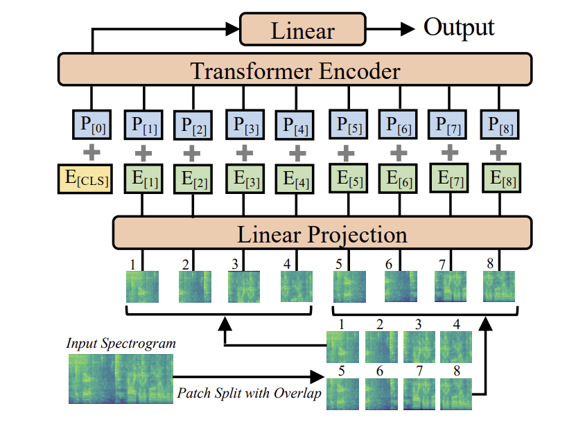
*Figure 10: AST Architecture. Source: [Gong et al., 2021] (https://arxiv.org/pdf/2104.01778)*
- The spectrogram is divided into overlapping patches
- Each patch is projected into a patch embedding
- Each patch embedding is added with a learnable positional embedding
- The patch sequence is fed into the transformer encoder
This representation allows audio signals to be processed using vision models such as Vision Transformers, and even enables CLIP-style training that aligns audio with text descriptions.
## 6 Modern Vision-Language Models
Recent systems extend CLIP by combining vision encoders with large language models.
Examples include:
- Flamingo: https://arxiv.org/abs/2204.14198
- BLIP / BLIP-2: https://arxiv.org/abs/2301.12597
- LLaVA: https://arxiv.org/abs/2304.08485
These systems enable tasks such as visual question answering, image captioning, and multimodal reasoning. While we do not cover these in this course, feel free to check them out!
## 7 References / Resources
- Dosovitskiy et al., 2021 - An Image is Worth 16x16 Words: Transformers for Image Recognition at Scale [https://arxiv.org/pdf/2010.11929]
- Liu et al., 2021 - Swin Transformer: Hierarchical Vision Transformer using Shifted Windows [https://arxiv.org/pdf/2103.14030]
- Medium - Distillation with NO Labels [https://medium.com/@ayyucedemirbas/distillation-with-no-labels-9e09b9b6dde2]
- Caron et al., 2021 - Emerging Properties in Self-Supervised Vision Transformers [https://arxiv.org/pdf/2104.14294]
- He et al., 2021 - Masked Autoencoders Are Scalable Vision Learners [https://arxiv.org/abs/2111.06377]
- Radford et al., 2021 - Learning Transferable Visual Models From Natural Language Supervision [https://arxiv.org/pdf/2103.00020]
- Gong et al., 2021 - AST: Audio Spectrogram Transformer [https://arxiv.org/pdf/2104.01778]
* https://prajnaaiwisdom.medium.com/emerging-datasets-for-vision-language-research-building-better-models-59f67f5fe8ea
* https://medium.com/one-minute-machine-learning/clip-paper-explained-easily-in-3-levels-of-detail-61959814ad13
* https://doi.org/10.48550/arXiv.2002.05709
* https://medium.com/@navendubrajesh/vision-language-models-an-introduction-37853f535415