---
title: Image-to-Image Models and Generative Adversarial Networks (GANs)
---
# Image-to-Image Models and Generative Adversarial Networks (GANs)
## Image-to-Image Tasks
Many important vision problems can be framed as image-to-image tasks, where the input is an image and the output is also an image (or an image-like map). Examples from the lecture include:
- **Image Super-resolution:** Taking a low-resolution image and producing a high-resolution version.
- **Semantic Segmentation:** Assigning a class label to every pixel in an image (e.g., cow, grass, tree, sky).
- **Satellite-to-Map Translation:** Converting aerial photographs into map representations.
These tasks share a common structure: the model receives an image of dimension $ (H, W, 3) $ and produces an output of dimension $ (H, W, C) $, where $ C $ depends on the task. For semantic segmentation with $ C $ classes:
$$f_\theta : \mathbb{R}^{H \times W \times 3} \longrightarrow \mathbb{R}^{H \times W \times C}$$
Instead of outputting a single integer label per pixel, the model outputs a vector of length $ C $ at each pixel location, representing class probabilities. The final segmentation map is obtained by taking the argmax across channels.
### Applications
- **Autonomous Driving:** Semantic segmentation enables vehicles to understand their surroundings by labeling every pixel as road, pedestrian, vehicle, etc.
- **Medical Imaging:** Segmentation models can identify tumors, organs, and other structures in CT scans and MRIs, assisting clinicians in diagnosis.
### Comparison to Image Classification
In image classification, the model produces a single image-level prediction (e.g., "cow"). In semantic segmentation, the model produces a pixel-level prediction — every pixel gets its own class label. This is a much denser prediction task that requires the network to maintain spatial resolution throughout processing.
---
## Building Image-to-Image Networks
### The Hourglass Architecture
A natural architecture for image-to-image tasks is the **hourglass** (encoder-decoder) CNN. The key design choices are:
- **Convolutions:** Allow parallel extraction of features for each spatial location.
- **Downsampling (encoder):** Reduces spatial dimensions using pooling or strided convolutions, which improves computational efficiency and increases the effective receptive field.
- **Upsampling (decoder):** Restores spatial dimensions back to the original input resolution to produce the output image/map.
The hourglass shape arises from progressively shrinking spatial dimensions while increasing channel depth (encoder), then progressively expanding spatial dimensions while decreasing channel depth (decoder).
### Upsampling Methods
Since the encoder downsamples the feature maps, the decoder needs to upsample them back to the original resolution. Several approaches exist:
**Unpooling (no learned parameters):**
- **Nearest Neighbor:** Each value is replicated to fill the larger output grid. Simple but introduces blocky artifacts.
- **Bed of Nails:** Places each value in the top-left corner of its output region and fills the rest with zeros.
Both approaches do not recover spatial information lost during downsampling.
**Max Unpooling:**
- During max pooling in the encoder, the positions of the maximum values are recorded.
- During max unpooling in the decoder, the values are placed back at those recorded positions, with zeros elsewhere.
- This creates corresponding pairs of downsampling and upsampling layers, helping preserve spatial information.
**Up-Convolution (Transposed Convolution):**
- A learned upsampling operation. Each input value is multiplied by a filter and placed into the output, with overlapping regions summed together.
- This is the most common upsampling approach in modern architectures because the filter weights are learnable parameters, allowing the network to learn the best way to upsample.
### The U-Net Architecture
The **U-Net** (Ronneberger et al., MICCAI 2015) is the foundational image-to-image architecture that adds **skip connections** to the hourglass design:
- **Skip connections** directly connect encoder layers to their corresponding decoder layers at the same spatial resolution.
- This allows the decoder to combine high-level semantic features (from deeper layers) with low-level spatial details (from earlier layers).
- The result is significantly improved prediction quality, especially at object boundaries and fine-grained details.
The three key ingredients of U-Net:
| Component | Purpose |
|---|---|
| Convolutions | Parallel feature extraction for each pixel |
| Hourglass shape | Efficiency via downsampling; larger receptive field |
| Skip connections | Preserve low-level details for sharper predictions |
### Encoder-Decoder Perspective
The U-Net can also be understood from an encoder-decoder perspective:
- **Encoder:** Maps an image to a low-resolution, semantically rich feature map. This is essentially a standard classification backbone like ResNet.
- **Decoder:** Maps the low-dimensional feature map back to an image or image-like output.
This mirrors the encoder-decoder structure used for text (e.g., transformers). Depending on the application, one can use just the encoder (for classification), just the decoder (for generation from a latent code), or both together (for image-to-image tasks).
### Autoencoders
An autoencoder is a special case of the encoder-decoder framework where the input and output are the same image. The encoder compresses the image into a low-dimensional latent vector (bottleneck), and the decoder reconstructs the original image from that vector. The latent space learned by the encoder captures meaningful structure — for example, when trained on MNIST digits, different digit classes tend to cluster in different regions of the latent space.
---
## Unpaired Image Translation
### The Problem with Paired Data
For supervised image-to-image tasks (e.g., segmentation), we need paired training data: each input image has a corresponding ground-truth output. However, for many translation tasks (e.g., horse → zebra, photo → painting), exact paired data does not exist. We only have two separate collections of images from each domain.
**The challenge:** Without paired ground truth, how can we tell if the model produced a good output?
### Using a Discriminator as a Learning Signal
The key insight is to train a **discriminator** — a binary classifier that determines whether a given image belongs to the target domain (e.g., "is this a real zebra image?"). This discriminator provides the learning signal that replaces paired supervision.
The discriminator is trained with binary cross-entropy loss:
$$\min_D \left[-y \log(D(\mathbf{x})) - (1-y)\log(1 - D(\mathbf{x}))\right]$$
where $ y = 1 $ for real target-domain images and $ y = 0 $ for generated images.
---
## Generative Adversarial Networks (GANs)
### Core Components
A GAN consists of two networks trained in opposition:
1. **Generator (G):** Produces images that should look like they belong to the target domain. For image-to-image translation, this can be parameterized as a U-Net.
2. **Discriminator (D):** A binary classifier that tries to distinguish real target-domain images from generated ones.

_Figure 1: The fundamental architecture of a Generative Adversarial Network, showing the generator producing fake images from random noise and the discriminator evaluating both real and generated images. Source: [Generative Adversarial Networks: A rivalry that strengthens](https://quantdare.com/generative-adversarial-networks-a-rivalry-that-strengthens/)_
### Adversarial Training
The training process is a minimax game:
- **Discriminator goal:** Correctly classify real images as real and generated images as fake.
- **Generator goal:** Fool the discriminator by producing images that it classifies as real.
**Per-sample objective:**
$$\max_G \min_D \left[-\log(D(\mathbf{x})) - \log(1 - D(G(\mathbf{z})))\right]$$
**Full objective over distributions:**
$$\max_G \min_D \left[\mathbb{E}_{\mathbf{x} \sim p_{\text{data}}}\left[-\log(D(\mathbf{x}))\right] + \mathbb{E}_{\mathbf{z} \sim p_z}\left[-\log(1 - D(G(\mathbf{z})))\right]\right]$$
### Training Procedure
Training alternates between two updates each iteration:
1. **Discriminator update:** Feed both real images and generated images to $ D $, compute classification loss, update $ D $'s weights to better distinguish real from fake.
2. **Generator update:** Generate images, pass them through $ D $ (with $ D $'s weights frozen), and backpropagate the derivative through $ D $ into $ G $, flipping the gradient sign so that $ G $ learns to produce outputs that $ D $ classifies as real.
Over the course of training, generated images progress from noise-like outputs to increasingly realistic samples. Ideally, the discriminator becomes "confused" (loss plateaus) as the generator's outputs become indistinguishable from real data.
---
## Issues with GANs and Solutions
### Issue #1: Vanishing Gradients with Strong Discriminator
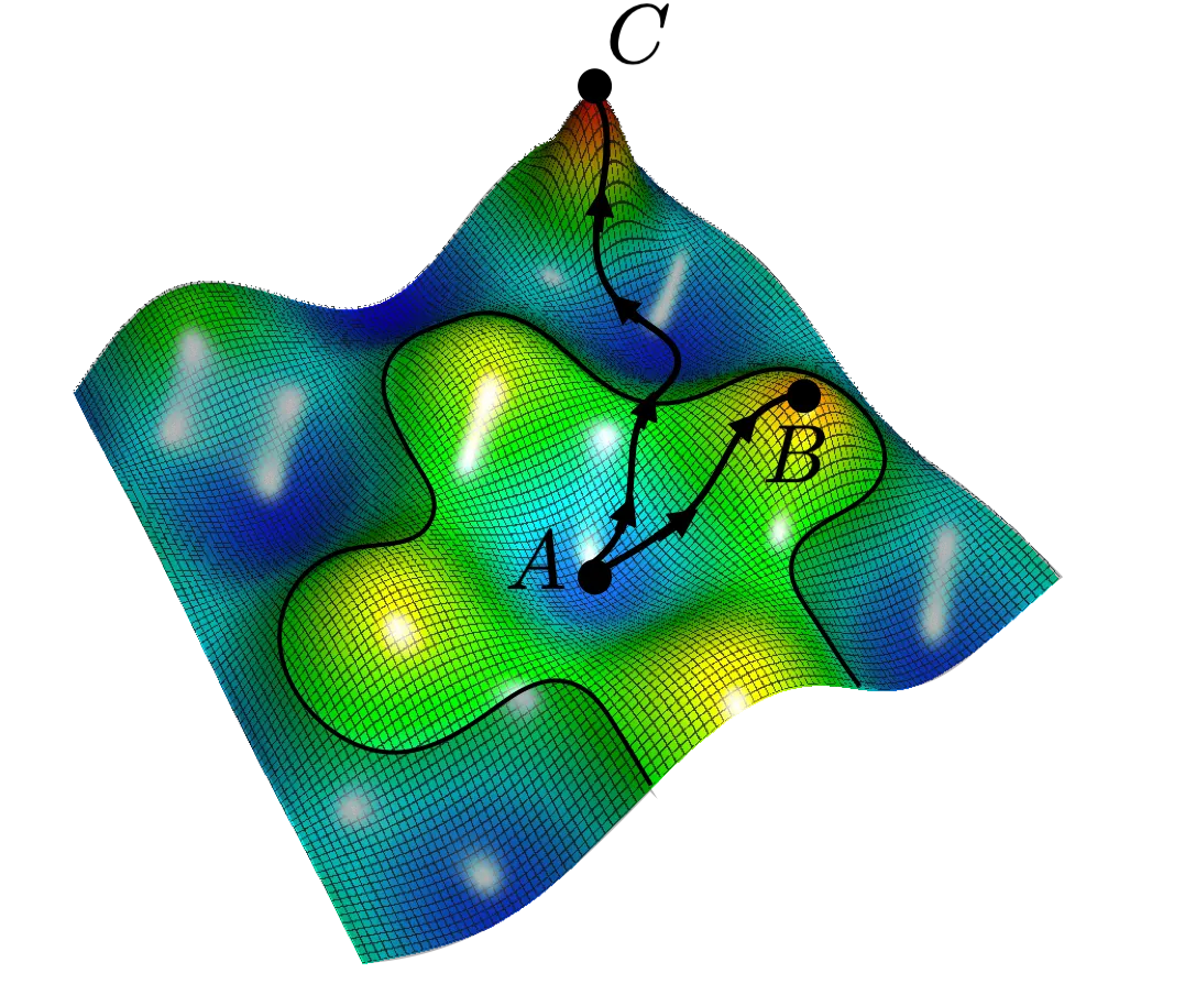
_Figure 2: Visualization of the minimax optimization landscape showing how the discriminator and generator objectives can lead to unstable training dynamics and potential convergence issues. Source: [Medium - WGAN-GP](https://jonathan-hui.medium.com/gan-wasserstein-gan-wgan-gp-6a1a2aa1b490)_
The minimax objective suffers from **vanishing gradients** when the discriminator becomes too strong. If $ D $ confidently classifies all generated images as fake (i.e., $ D(G(\mathbf{z})) \approx 0 $), then $ \log(1 - D(G(\mathbf{z}))) \approx 0 $, and the gradient signal to $ G $ vanishes. The generator receives no useful learning signal.
**Solution — Modified (Non-Saturating) Loss:**
Instead of minimizing the probability of being classified as fake, the generator maximizes the probability of being classified as real:
| Original (minimax) | Modified (non-saturating) |
|---|---|
| $ \min_G \log(1 - D(G(\mathbf{z}))) $ | $ \min_G -\log(D(G(\mathbf{z}))) $ |
| = minimize discriminator predicting **fake** | = maximize discriminator predicting **real** |
The modified loss provides much stronger gradients early in training when the generator is still poor, because $ -\log(D(G(\mathbf{z}))) $ has a steep slope near $ D(G(\mathbf{z})) = 0 $.
### Issue #2: Mode Collapse
**Mode collapse** occurs when the generator fails to capture the full diversity of the data distribution and instead "collapses" to producing a limited variety of outputs that reliably fool the discriminator.
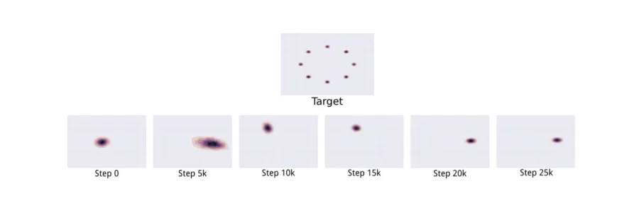
_Figure 3: Illustration of distribution of generated samples that shows mode collapse in GANs — the generator concentrates on a subset of modes rather than covering the full target distribution. Source: [Medium - Mode Collapse](https://medium.com/@miraytopal/what-is-mode-collapse-in-gans-d3428a7bd9b8)_
For example, when training on a dataset of dogs and cats, the generator might specialize in producing only realistic dogs while completely ignoring cats — it still successfully fools the discriminator but has failed to model the full distribution.
Formally, if $ S_k $ represents the support of mode $ k $ in the data distribution, mode collapse occurs when the generator's distribution $ p_g $ assigns near-zero probability to some modes while concentrating on others.
**Causes include:**
- The discriminator becoming too strong, pushing the generator toward "safe" outputs
- Optimization dynamics that favor certain modes over others
- Insufficient generator capacity
### Issue #3: Information Preservation in Unpaired Translation
For unpaired image translation (e.g., horse → zebra), a standard GAN discriminator only ensures the output *looks like* a zebra. It does not ensure the output preserves the content/structure of the input image. The generator could produce any valid zebra image regardless of the input horse's pose, background, etc.
**Solution — Cycle Consistency (CycleGAN):**
The key idea from Zhu et al. (ICCV 2017) is that image translation should be **invertible**: translating a horse to a zebra and then back to a horse should recover the original image.

_Figure 4: Illustration of cycle consistency constraint in CycleGAN showing how image translation should be invertible — translating from domain A to B and back to A should recover the original image. Source: [HaikuTechCenter](https://www.haikutechcenter.com/2020/11/cyclegan-gan-architecture-for-learning.html)_
CycleGAN trains two generators:
- $ G_1 $: maps domain A → domain B (e.g., horse → zebra)
- $ G_2 $: maps domain B → domain A (e.g., zebra → horse)
And enforces a **cycle consistency loss** (reconstruction loss):
$$\mathcal{L}_{\text{cycle}} = \|\mathbf{x}_{\text{horse}} - G_2(G_1(\mathbf{x}_{\text{horse}}))\|_2^2$$
The total CycleGAN loss combines:
- **Discriminator loss:** Ensures generated images look realistic in the target domain
- **Reconstruction loss:** Ensures content and structure are preserved through the translation cycle
**Applications of unpaired translation:**
- Style transfer (photo → Monet, Van Gogh, Cezanne, Ukiyo-e styles)
- Season transfer (summer → winter)
- Domain adaptation for training data augmentation
---
## Unconditional Generation with GANs
GANs can also perform **unconditional generation** — generating images from scratch without any input image. Instead of translating from a source image, the generator takes **random Gaussian noise** $ \mathbf{z} $ as input and produces an image:
$$\tilde{\mathbf{x}} = G(\mathbf{z}), \quad \mathbf{z} \sim \mathcal{N}(0, I)$$
### Latent Space Properties
The Gaussian noise vector $ \mathbf{z} $ is not arbitrary — it develops meaningful structure during training:
- **Similar noise vectors produce similar images:** Small perturbations in $ \mathbf{z} $ lead to small changes in the output.
- **Noise dimensions become meaningful:** Different dimensions can correspond to different semantic attributes (e.g., pose, hair color, expression).
- **Style mixing:** By using different parts of the latent vector at different layers (as in StyleGAN), one can combine coarse attributes from one sample with fine details from another.
This structure enables controlled generation by manipulating the latent vector.
---
## Recap
- Many vision tasks (segmentation, super-resolution, etc.) can be formulated as **image-to-image problems**.
- The **U-Net** is a versatile encoder-decoder architecture with skip connections for these tasks.
- **Unpaired image translation** uses a discriminator as a learning signal when paired data is unavailable.
- **GANs** train a generator and discriminator adversarially. Three key issues arise:
1. **Vanishing gradients** with a strong discriminator → solved by the non-saturating loss
2. **Mode collapse** → the generator fails to capture full data diversity
3. **Information preservation** → solved by cycle consistency (CycleGAN)
- GANs can perform **unconditional generation** from Gaussian noise, with meaningful latent space structure.
---
## Optional: Advanced Topics
*The following topics extend beyond the core lecture material but provide deeper context for interested students.*
### Optional: Information Theory Perspective
The optimal discriminator computes the Bayes-optimal classifier:
$$D^*(\mathbf{x}) = \frac{p_{\text{data}}(\mathbf{x})}{p_{\text{data}}(\mathbf{x}) + p_g(\mathbf{x})}$$
This reveals that the discriminator performs density ratio estimation between the true data distribution $ p_{\text{data}} $ and the generated distribution $ p_g $. The GAN objective is closely related to minimizing the Jensen-Shannon divergence between these distributions.
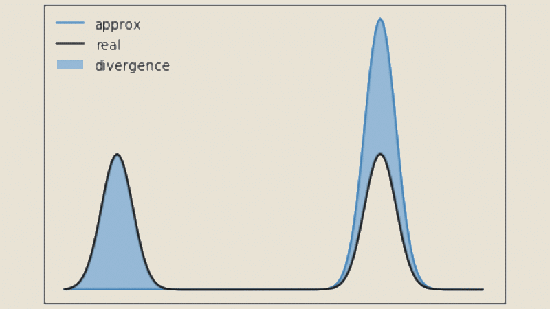
_Figure 5: Visual representation of Jensen-Shannon divergence between two probability distributions. The discriminator's optimization process aims to minimize this divergence between the real data distribution and the generated distribution. Source: [DataScientest - Jensen-Shannon Divergence](https://datascientest.com/en/jensen-shannon-divergence-everything-you-need-to-know-about-this-ml-model)_
### Optional: Discriminator Architecture — PatchGAN
Rather than outputting a single scalar for the entire image, a **PatchGAN** discriminator produces a matrix of local predictions:
$$D(\mathbf{x}) \in \mathbb{R}^{H/k \times W/k \times 1}$$
Each element represents the probability that a specific local patch is real. This provides spatially-specific feedback and reduces parameter count.

_Figure 6: The PatchGAN structure in the discriminator architecture showing how local patches are evaluated independently to produce a matrix of decisions rather than a single global classification. Source: [ResearchGate - PatchGAN](https://www.researchgate.net/figure/The-PatchGAN-structure-in-the-discriminator-architecture_fig5_339832261)_
### Optional: Multi-scale Discriminators
Multiple discriminator networks operate at different resolutions:
$$\mathcal{L}_{\text{multiscale}} = \sum_{k=0}^{K} \lambda_k \mathcal{L}_{\text{GAN}}(G, D_k)$$
where $ D_k $ processes images downsampled by factor $ 2^k $. This allows simultaneous evaluation of fine details and global structure.

_Figure 7: Example of multi-scale and multi-level discriminator architecture showing how the discriminator processes images at different resolutions simultaneously. Source: [ResearchGate - Multi-scale Discriminator](https://www.researchgate.net/figure/The-example-of-multiscale-and-multilevel-discriminator-There-are-three-columns-which_fig2_329536290)_
### Optional: StyleGAN Architecture
StyleGAN introduces several innovations for high-quality unconditional generation:

_Figure 8: StyleGAN generator architecture showing the complete flow from input noise z through the mapping network to the synthesis network with progressive generation. Source: [Medium - StyleGAN Explained](https://medium.com/@arijzouaoui/stylegan-explained-3297b4bb813a)_
1. **Mapping Network:** An 8-layer MLP maps random noise $ z $ to an intermediate latent space $ w = f(z) $, which exhibits better disentanglement of semantic attributes.
2. **Style Modulation (AdaIN):** The latent code $ w $ controls adaptive instance normalization at each layer:
$$\text{AdaIN}(x_i, y) = y_{s,i} \frac{x_i - \mu(x_i)}{\sigma(x_i)} + y_{b,i}$$
3. **Progressive Generation:** The network builds images from low to high resolution, with each resolution responsible for different levels of detail.
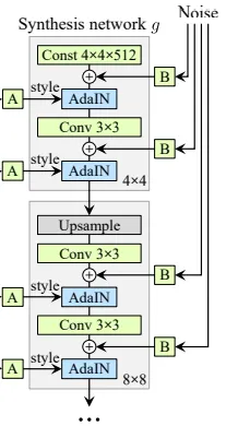
_Figure 9: Detailed view of the StyleGAN synthesis network block showing how style modulation (A) and noise injection affect feature generation at each layer. Source: [Medium - StyleGAN Explained](https://medium.com/@arijzouaoui/stylegan-explained-3297b4bb813a)_
### Optional: Training Stabilization — WGAN-GP
The Wasserstein GAN with Gradient Penalty enforces Lipschitz continuity through gradient constraints:
$$\mathcal{L}_{GP} = \lambda \mathbb{E}_{\hat{\mathbf{x}}}\left[\left(\|\nabla_{\hat{\mathbf{x}}} D(\hat{\mathbf{x}})\|_2 - 1\right)^2\right]$$
where $ \hat{\mathbf{x}} $ is a random interpolation between real and fake samples. This eliminates weight clipping artifacts and provides consistent gradient magnitude throughout training.
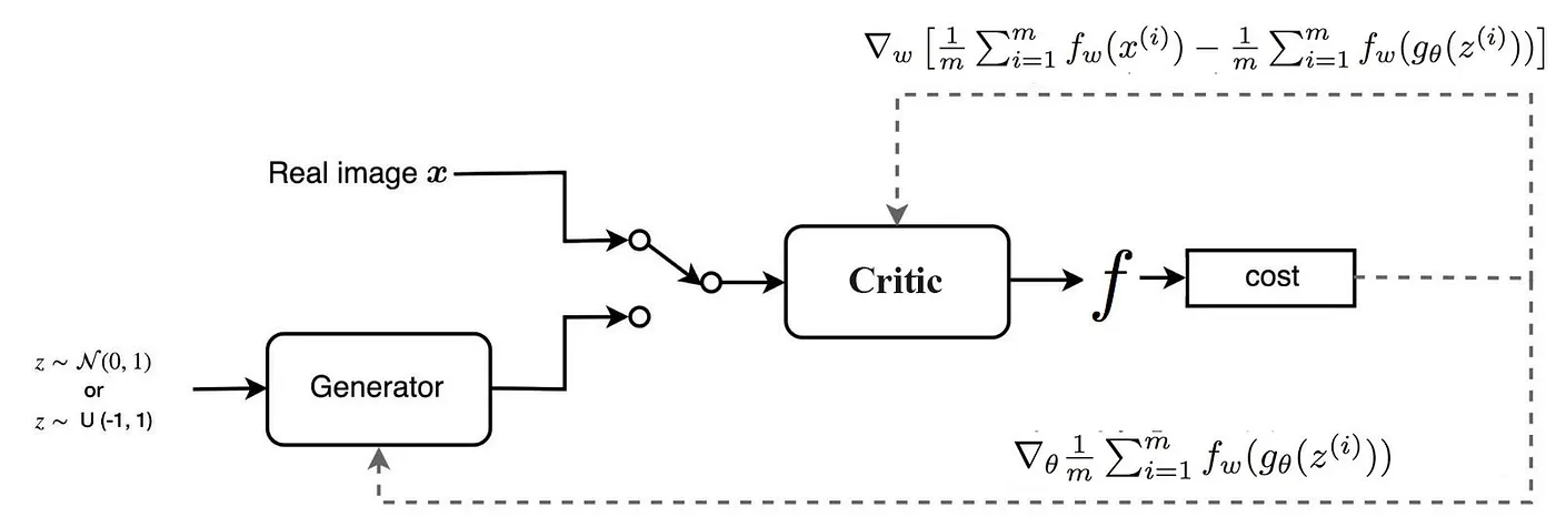
_Figure 10: Illustration of WGAN-GP gradient penalty mechanism showing how gradients are computed on interpolated points between real and fake samples to enforce smooth transitions. Source: [Medium - WGAN-GP](https://jonathan-hui.medium.com/gan-wasserstein-gan-wgan-gp-6a1a2aa1b490)_
### Optional: BigGAN
BigGAN scaled up GAN architectures with orthogonal regularization ($ \mathcal{L}_{\text{ortho}} = \beta \sum_i \|W_i^T W_i - I\|_F^2 $), class-conditional batch normalization, hierarchical latent spaces, and self-attention mechanisms for large-scale, high-quality generation.
### Optional: Few-shot GANs
Adapting pretrained GANs to new domains with minimal data using techniques like freezeout (gradually freezing discriminator layers), feature matching, and elastic weight consolidation to prevent catastrophic forgetting.

_Figure 11: Real images (left) and few-shot GAN generated images (right), demonstrating GAN adaptation with limited training data. Source: [ResearchGate](https://www.researchgate.net/figure/Real-images-left-and-few-shot-GANs-generated-images-right-where-the-left-image-is_fig1_338187408)_
### Optional: GANs for 3D Generation
Three-dimensional GANs use 3D convolutions for volumetric data and projection discriminators for multi-view consistency. Applications include medical image reconstruction, molecular structure generation, and 3D object synthesis.
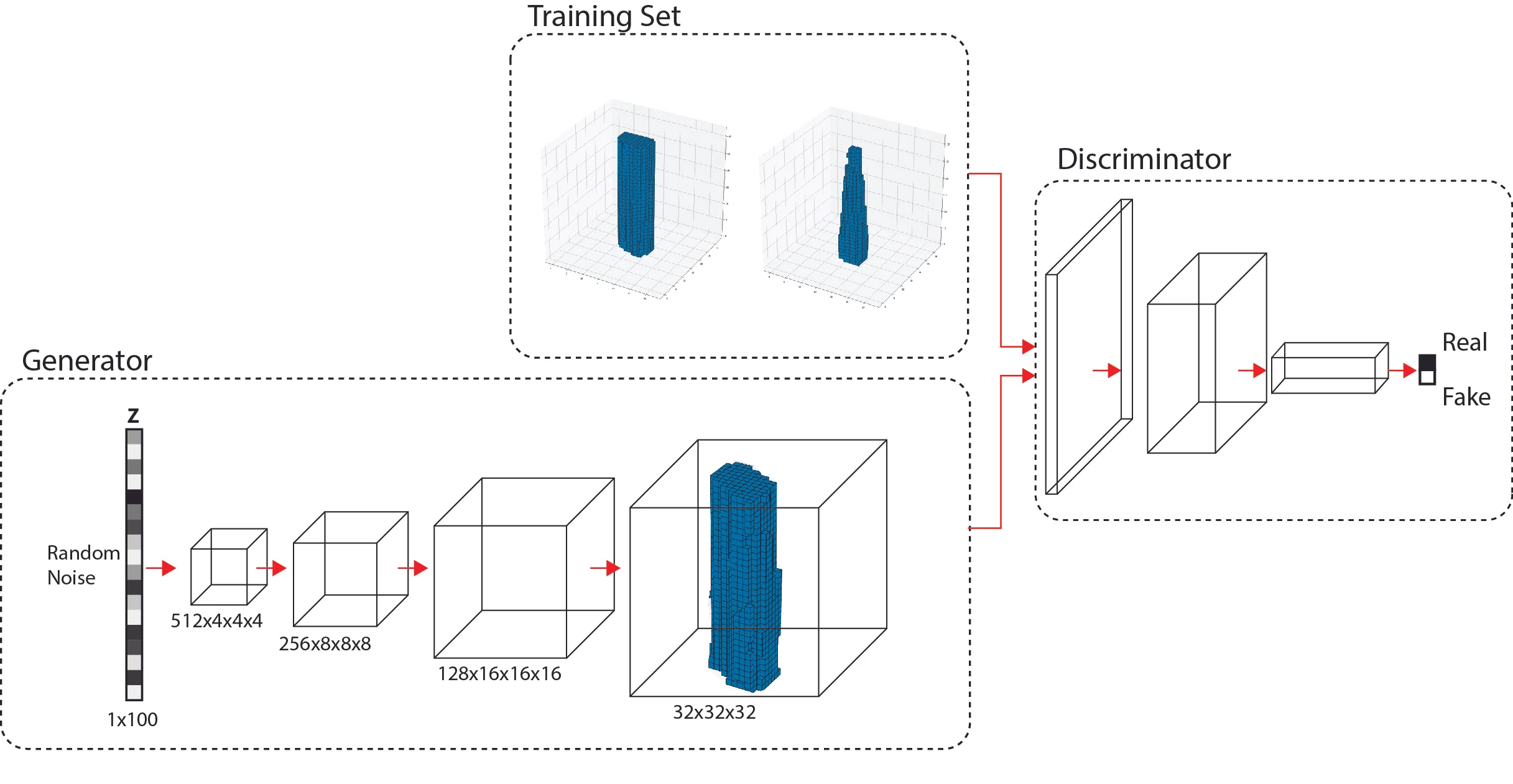
_Figure 12: Illustration of 3D GAN Architecture generating volumetric objects. Source: [Computational Architecture Lab - 3D Generative Adversarial Networks](https://www.computationalarchitecturelab.org/3d-generative-adversarial-networks)_