---
title: Variational Autoencoders (VAEs)
---
# Variational Autoencoders (VAEs)
Edited notes originally from Akanksha Sarkar (as2637) and Ian Yang (ijy2), based on Cornell CS 4782 Spring 2025.
## Discriminative vs. Generative Models Review
- **Discriminative models**: These are models which aim to model $ p(Y|X) $ and are used to predict labels given data. E.g. classifying images of digits (0–9) based on pixel values.
- Since they require labeled data, they are typically **supervised**
- We have seen them in the form of: Logistic regression, NNs with softmax layers, SVMs, etc
- **Generative models**: These are models which aim to model $ p(X) $ and instead of trying to predict some associated label, they aim to generate new data that looks like the training data.
- Since we do not require labels, this is unsupervised in nature.
- Examples of such models include:
- Generative Adversarial Networks (GANs)
- Variational Autoencoders (VAEs)
- Diffusion Models
- **Conditional Generative models**: These models aim to generate new data samples based on some input condition or context, such as a label or prompt. Instead of sampling from the full data distribution $ p(X) $, the model learns to generate samples from $ p(X \mid Y) $, where $ Y $ is the condition. This allows for controlled generation—for example, creating images of specific digits or generating text with a desired prompt.
### Big Picture Idea of Generating new data
There are three main steps involved in trying to generate new data from existing data samples:
1. **Data Sampled from True $ P(X) $**: We first observe data (e.g., MNIST digits) sampled from the real but unknown distribution $ P(X) $ of data points. This distribution is usually complex and high-dimensional.
2. **Learn Approximate Distribution $ Q(X) $**: The model (e.g., a VAE) learns a simpler distribution $ Q(X) $ that mimics the true one. This is the training phase, where the model tries to capture the patterns and variations in real data it observes.
3. **Use $ Q(X) $ to generate new data**:After training, we sample from $ Q(X) $ to generate new, artificial data. If $ Q(X) \approx P(X) $, then these samples will look like real data.
### Data Manifolds
Now we will introduce some math terminology (don't be scared though, this is intuitive). A manifold is a collection/set of points that lie in a space (called the ambient space), such as $ \mathbb{R}^n $. The shape of a manifold could be anything (a blob, a wavy surface, a cinnamon roll, etc).
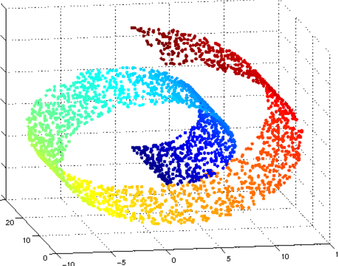
The **dimension of a manifold** is given by how many dimensions a local patch the manifold has. For example, the manifold/cinnamon roll above is a 2 dimensional manifold because locally (zooming in on a point) it looks like a 2D-plane. This manifold lies in 3D space as seen in the image.
A **data manifold** is a manifold where each point corresponds to a valid data example. For example, imagine in the image above that each point on the cinnamon roll represents a unique 28 x 28 image of a handwritten digit. While the ambient space contains all possible 28 x 28 images, only a small subset of the points in the ambient space correspond to **realistic** handwritten digits. These valid images are what make up the lower-dimensional data manifold.
Because the data manifold occupies only a small region of the ambient space, randomly sampling points from the ambient space almost always gives points lying off the manifold. In the handwritten digit example, most randomly generated pixel arrays will look like noise rather than meaningful digits.
One way to solve this problem includes **sampling from a simple prior distribution like a Gaussian distribution** (which we know how to sample from easily), and then learn a mapping from that Gaussian space to the image manifold.
This is essentially what VAEs and GANs do:
- VAEs learn a smooth, probabilistic mapping between latent Gaussian variables and image data.
- GANs learn to transform noise vectors (usually sampled from the normal gaussian distribution) into realistic samples through adversarial training.
Therefore, to generate valid data (e.g. MNIST digits), we must avoid sampling directly in image space. Instead, we map from a known distribution (like a Gaussian) into the narrow, structured image manifold where real data lives.
### A little history...
VAE is the original Generative model! (a trendsetter if you must...)
- **VAEs (2013)** were the first major deep generative models, introduced by *Kingma & Welling*. They used a probabilistic latent space to generate data.
- **GANs (2014)** were introduced by *Goodfellow et al.* and aimed to fix some shortcomings of VAEs (especially the blurry outputs).
- **Diffusion Models (2015)** were introduced by *Sohl-Dickstein et al*.These models use iterative denoising processes and have become the state-of-the-art in image generation (e.g., Stable Diffusion, DALL·E 3).
## Dimensionality Reduction
The core concept behind VAEs is: reducing high-dimensional data to a low-dimensional latent representation.
- As mentioned before, real-world data (like images) often lies on a low-dimensional manifold, in a high-dimensional space.
- Our goal is to map the given high-dimensional input $ x \in \mathbb{R}^D $ to a lower-dimensional latent variable $ z \in \mathbb{R}^d $, where $ d \ll D $.
Dimensionality reduction is useful for:
- **Visualization**: Helps us plot and understand the structure of data.
- **Feature Extraction**: Lower-dimensional representations often capture the most important information, useful for tasks like classification.
- **Understanding Relationships**: The latent space can reveal clusters, structure, or smooth transitions between data points.
- **Sampling**: In generative models like VAEs, we want to sample in this latent space and generate new data.
So we know that the mapping from $ x \to z $ is really useful. Next we will examine what the nature of this mapping. Consider the following question:
> **What properties should the mapping $ x \to z $ have?**
Some properties you might consider are:
- The mapping should preserve key semantic or structural information.
- It should have enough information that we can go back to $ x $ from $ z $.
- In case of VAEs, it should make sampling easy (so that we can generate new data easily!)
Essentially, dimensionality reduction helps us compress complex data into a simpler form that’s still meaningful. VAEs learn this kind of mapping to enable both data understanding and generation.
One common dimensionality reduction technique you have probably seen before is PCA.
### Principal Component Analysis (PCA)
The main assumption when using PCA is that the data lies near a linear subspace within the high-dimensional space.
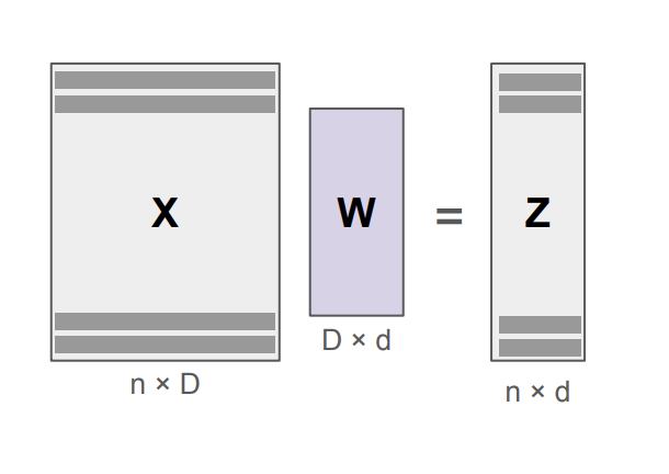
- **Encoding step** This involves projecting given data into lower-dimensional space:
$ \mathbf{z} = \mathbf{W}(\mathbf{x} - \boldsymbol{\mu}) $
where $ \mathbf{W} $ is a projection matrix and $ \mu $ is the data mean.
- **Decoding step** This involves getting the original data back from the encoded z:
$ \mathbf{x} \approx \mathbf{W}^\top \mathbf{z} + \boldsymbol{\mu} $
The goal here is to choose $ \mathbf{W} $ such that it captures maximum variance in the data. To do so:
- PCA finds the top eigenvectors of the data’s (centered) covariance matrix $ \mathbf{X} \mathbf{X}^\top $.
- These eigenvectors define the directions of maximum variance or the **principal components**.
PCA is **linear**, simple, and fast to compute using linear algebra. In our discussion it serves as a baseline for learning more complex (nonlinear) dimensionality reduction techniques like autoencoders and VAEs.
- While PCA is useful for **visualization and feature extraction**, it can’t capture **nonlinear** structures in the data. This is a major problem because in general, **data manifolds are nonlinear**.
Next we will examine a non-linear dimensionality reduction method.
## Autoencoders
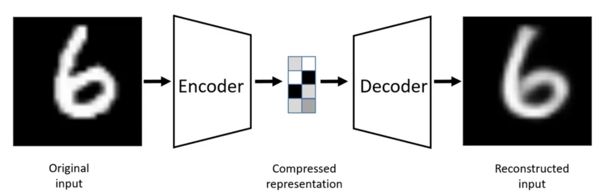
Autoencoders were first introduced by Kramer (1991) and use neural networks for **non-linear dimensionality reduction**. They do this in a two step process: first, by learning to compress data into a lower-dimensional space and then secondly reconstruct it back, ideally preserving the original information.
The architecture (following the two steps) is also divided into two components:
- **Encoder** $ e(x) $: maps input data $ x \in \mathbb{R}^D $ to a latent variable $ z \in \mathbb{R}^d $
- **Decoder** $ d(z) $: maps back from the latent space to reconstruct $ x' \approx x $
The latent representation is $ z $ which captures a compressed representation ideally preserving important features.
### Loss Function
Since the goal is to have a meaningful latent representation, one way to test whether $ z $ is meaningful is to check if it contains enough information to construct the original $ x $ from it.
The goal is therefore to **minimize reconstruction error**:
$$\min_{\phi, \theta} \sum_{x \in \mathcal{D}} \| x - x' \|^2 \quad \text{where} \quad x' = d_\theta(e_\phi(x))$$
- $ \phi $ is encoder parameters, $ \theta $ is decoder parameters
- **Common losses**: Mean squared error (MSE), or absolute loss
- Notice that the loss encourages $ x' $ to be as close as possible to the original $ x $.
The idea is similar to "cycle consistency" used in models like CycleGAN: If you can encode and decode something and get back the same input, the model likely captured meaningful structure.
The encoder, decoder structure can be really powerful. However, you might want to consider what happens when both encoder and decoder are linear?
- *Spoiler* : The model reduces to PCA.
Therefore we should keep this in mind when trying to figure out the properties of $ e(x) $ and $ d(z) $. Having said that, consider the next question:
> What properties should $ e(x) $ and $ d(z) $ have?
Some peoperties you might consider:
- Non-linearity (to capture complex structure)
- Smoothness and continuity
- Ability to generalize and reconstruct unseen inputs
### Sampling from Autoencoders
We’d like to generate new data by sampling $ z \sim P(z) $ and feeding it into the decoder $ d(z) $. However, in order to do so we must ensure the latent space has a known structure (e.g., Gaussian), so it’s easy to sample from. Without such structure, randomly sampled $ z $ values may map to nonsensical outputs. This leads us to:
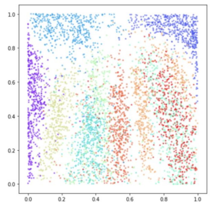
#### Problem with Autoencoders
Consider the following graph showing the latent space learned by an autoencoder trained on the MNIST dataset. Each point corresponds to an input digit, and colors indicate the digit class (0–9). The scatterplot shows that while some digits form distinct clusters, the overall structure is uneven, with significant empty regions and overlap between digit groups. This “naive” latent space is therefore not ideal because it lacks a sense of continuity which makes it hard to generate meaningful new samples by picking random points.
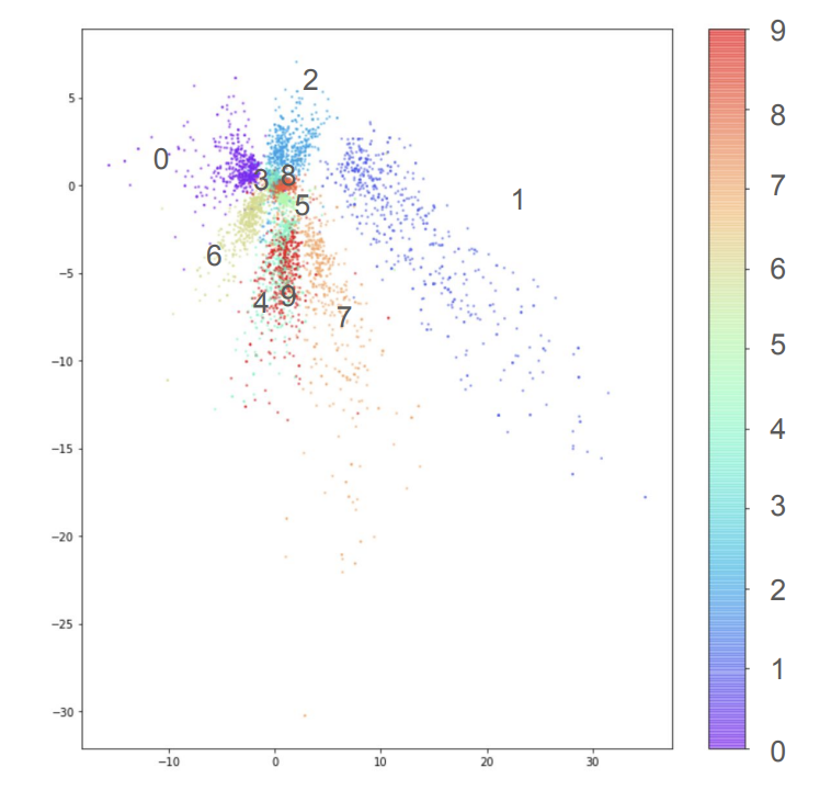
More generally, we face the following problems with regular autoencoders:
- The learned latent space tends to be:
- **Sparse**: There are lots of empty space
- **Unstructured**: For example, in the MNIST dataset, the digits cluster unevenly.
All these properties of the latent space make it difficult to sample new $ z $ and get meaningful outputs i.e. generation from autoencoders unreliable.
Given that motivation, we are almost ready to delve into Variational Autoencoders! However, it can become a bit math heavy so lets make sure we have our probability basics clear.
### Some background on probability fundamentals
## Probability and Information: Foundations for VAEs
Understanding Variational Autoencoders (VAEs) requires some fundamental concepts from probability theory. These concepts help formalize how we represent uncertainty, model data, and compare distributions.
### Conditional and Marginal Probabilities
The joint probability of two random variables $ X $ and $ Y $ can be factorized using the chain rule:
$$p(X, Y) = p(Y \mid X) \cdot p(X)$$
To compute the marginal probability $ p(X) $, we integrate over the other variable:
$$ p(X) = \int p(X, y) \, dy$$
### Joint and conditional distributions
$$ p(\mathbf{x}) = \frac{p(\mathbf{x}, \mathbf{z})}{p(\mathbf{z} \mid \mathbf{x})} $$
This expression will reappear in the derivation of the Evidence Lower Bound (ELBO) in VAEs.
### Surprisal and Log-Likelihood
**Surprisal**, measures how "unexpected" an event is under a given probability distribution. For a sample $ x $ drawn from a model with parameters $ \theta $, the surprisal is defined as:
$$\text{Surprisal}(x) = -\log p_\theta(x)$$
Minimizing surprisal is equivalent to minimizing the negative log-likelihood, which is also equivalent to maximizing the log-likelihood:
$$\min_\theta \log \left( \frac{1}{p_\theta(x)} \right) = \min_\theta \left( -\log p_\theta(x) \right) = \max_\theta \log p_\theta(x)$$
---
### KL Divergence
The Kullback-Leibler (KL) Divergence measures how much one probability distribution $ q(x) $ (the model) differs from another probability distribution $ p(x) $ (the reference or reality):
$$D_{\text{KL}}(p \parallel q) = \mathbb{E}_{x \sim p} \left[ \log \frac{p(x)}{q(x)} \right]$$
KL divergence can be viewed as the difference between the cross-entropy and the entropy:
$$\mathbb{E}_{x \sim p} \left[ \log \frac{1}{q(x)} \right] - \log \frac{1}{p(x)}$$
#### Properties:
- Non-negative: $ D_{\text{KL}}(p \parallel q) \geq 0 $
- Zero if and only if $ p = q $
- Not symmetric: $ D_{\text{KL}}(p \parallel q) \neq D_{\text{KL}}(q \parallel p) $
#### Intuition Behind KL Divergence
Consider two coins with different biases. Coin A is standard, while coin B is biased (e.g., more likely to land heads). Is it equally easy to mistake coin A for coin B as mistaking coin B for coin A? The answer is **no**, it is not equally easy. KL divergence $ D_{\text{KL}}(P \parallel Q) $ measures how well distribution Q (e.g., the model) approximates distribution P (e.g., the true data). Mistaking a rare event for a common one is less costly than the reverse, and KL divergence penalizes such mismatches unevenly. This is why KL divergence is not symmetric.
Finally, we are ready to delve into VAEs! We will first start by making specific parts of the Autoencoder probabilistic in nature.
## Making Autoencoders Probabilistic
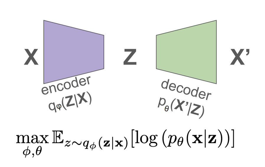
To make an autoencoder probabilistic, we replace its deterministic encoder and decoder with probabilistic mappings. Instead of mapping an input $ x $ to a fixed latent vector $ z $, we define a distribution over $ z $ given $ x $, denoted $ q_\phi(z \mid x) $. Similarly, the decoder models the likelihood of reconstructing $ x $ from $ z $ via $ p_\theta(x \mid z) $.
The training objective is to maximize the expected log-likelihood of the reconstruction, i.e., the expected probability of recovering $ x $ after encoding and decoding it.
So far the we have used softmax can be to produce probabilities, however notice that softmax will produce a discrete output space. Since we want a continuous latent space (for ease of sampling), it is more appropriate to model $ q_\phi(z \mid x) $ as a Gaussian distribution.
### Making the Encoder probabilistic
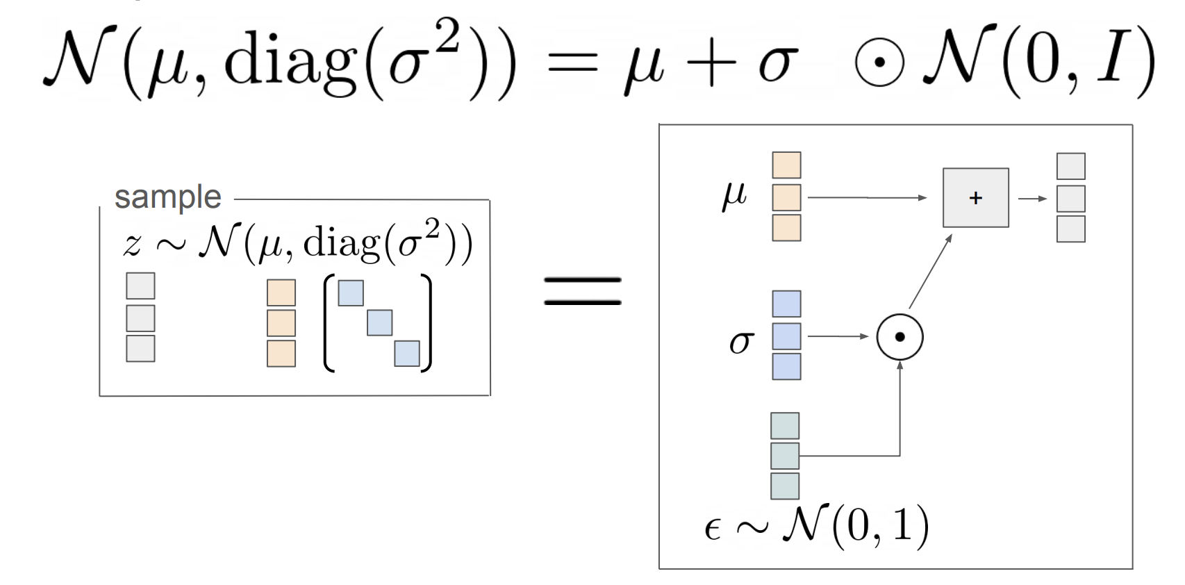
To model the encoder probabilistically, we assume that the latent variable $ z $ is sampled from a Gaussian distribution whose mean $ \mu $ and log-variance $ \log \sigma^2 $ are predicted by the encoder network:
$$
z \sim \mathcal{N}(\mu, \text{diag}(\sigma^2))
$$
However, this introduces a challenge: **we cannot backpropagate through a random sampling operation!** To address this, we use the **reparameterization trick**, which expresses $ z $ as a deterministic function of a noise variable:
$$
z = \mu + \sigma \cdot \epsilon, \quad \epsilon \sim \mathcal{N}(0, I)
$$
By sampling $ \epsilon $ from a standard normal distribution and treating $ \mu $ and $ \sigma $ as differentiable outputs of the encoder, we can propagate gradients through the computation graph. This allows us to train the model end-to-end using standard gradient-based optimization.
### Making the Decoder probabilistic
To complete the VAE architecture, we also make the decoder probabilistic. Given a latent variable $ z $, the decoder no longer outputs a single reconstruction $ x' $ directly. Instead, it defines a distribution over possible reconstructions. Specifically, we assume:
$$
x' \sim \mathcal{N}(d_\theta(z), \tau^2)
$$
The likelihood of observing a particular reconstruction $ x' $ under this distribution is:
$$
p_\theta(x' \mid z) \propto \exp\left( -\frac{(x' - d_\theta(z))^2}{\tau^2} \right)
$$
Taking the log of this expression and dropping constants, the log-likelihood becomes:
$$
\log p_\theta(x' \mid z) = -\frac{1}{\tau^2}(x' - d_\theta(z))^2 + \text{const}
$$
So, **maximizing the log-likelihood is equivalent to minimizing the squared reconstruction error**:
$$
\max_{\phi, \theta} \, \mathbb{E}_{z \sim q_\phi(z \mid x)} \left[ \log p_\theta(x \mid z) \right]
\quad \Leftrightarrow \quad
\min_{\phi, \theta} \, \mathbb{E}_{z \sim q_\phi(z \mid x)} \left[ (x - d_\theta(z))^2 \right]
$$
This shows how the probabilistic decoder leads to the familiar squared loss, but now justified through a likelihood-based probabilistic model. Our finished model looks like the figure below:
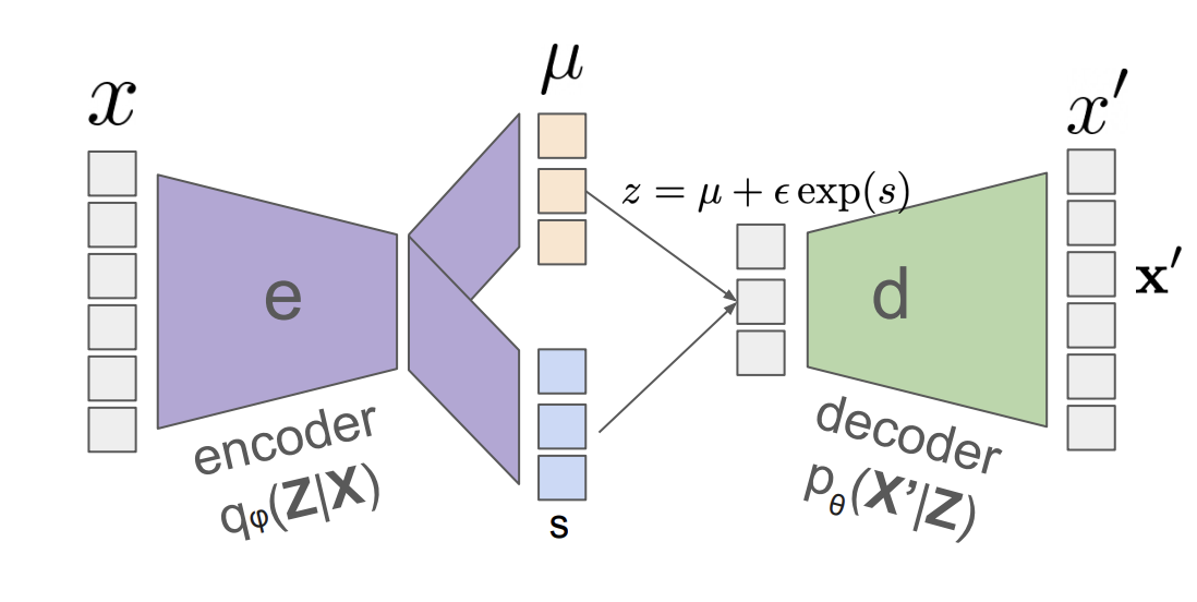
### Sampling from latent space
In a VAE, each input $ x $ is mapped to its own latent distribution $ q_\phi(z \mid x) $, typically a Gaussian with its own mean and variance. This poses a challenge: if every training point has its own latent region, how can we sample meaningful $ z $ values at test time, when we no longer have access to $ x $?
The solution is to constrain all the individual latent distributions to be *close to a shared prior*, typically a **standard normal distribution**:
$$
p(z) = \mathcal{N}(0, I)
$$
This is enforced by minimizing the KL divergence between the encoder distribution and the prior:
$$
D_{\text{KL}}(q_\phi(z \mid x) \, \| \, p(z))
$$
By regularizing $ q_\phi(z \mid x) $ to stay near $ p(z) $ for all $ x $, we ensure that samples drawn from $ p(z) $ (i.e., standard Gaussian noise) are meaningful and lie in regions where the decoder has been trained to reconstruct. This is what allows us to generate new samples by simply drawing $ z \sim \mathcal{N}(0, I) $ and passing it through the decoder:
$$
x' = d_\theta(z)
$$
The complete VAE objective combines this **prior-matching term** with the **reconstruction term**:
$$
\mathbb{E}_{q_\phi(z \mid x)}[\log p_\theta(x \mid z)] - D_{\text{KL}}(q_\phi(z \mid x) \, \| \, p(z))
$$
This ensures that the latent space is both informative for reconstruction and structured enough to sample from.
## Evidence Lower Bound (ELBO)
### ELBO Derivation
We want to compute or approximate the **marginal likelihood** (or evidence) $ \log p(x) $. Since this integral is often intractable, we derive a lower bound on it using variational inference.
We start with:
$$
\log p(x) = \log p(x) \int 1 \, dz \quad
$$
We know sum over probability distribution is 1, thus:
$$
\log p(x) = \log p(x) \int q_\phi(z \mid x) \, dz \quad
$$
Move $ \log p(x) $ inside the integral:
$$
= \int q_\phi(z \mid x) \log p(x) \, dz \quad
$$
Express as expectation (using the definition of expectation):
$$
= \mathbb{E}_{q_\phi(z \mid x)} [\log p(x)] \quad
$$
Apply identity: $ \log p(x) = \log \frac{p(x, z)}{p(z \mid x)} $:
$$
= \mathbb{E}_{q_\phi(z \mid x)} \left[ \log \frac{p(x, z)}{p(z \mid x)} \right] \quad
$$
Multiply and divide by $ q_\phi(z \mid x) $:
$$
= \mathbb{E}_{q_\phi(z \mid x)} \left[ \log \frac{p(x, z) \, q_\phi(z \mid x)}{p(z \mid x) \, q_\phi(z \mid x)} \right]
$$
Now using log properties, we can split the log:
$$\mathbb{E}_{q_\phi(z \mid x)} \left[ \log \frac{p(x, z)}{q_\phi(z \mid x)} \right] + \mathbb{E}_{q_\phi(z \mid x)} \left[ \log \frac{q_\phi(z \mid x)}{p(z \mid x)} \right]$$
The second term is the KL divergence:
$$
= \mathbb{E}_{q_\phi(z \mid x)} \left[ \log \frac{p(x, z)}{q_\phi(z \mid x)} \right] + D_{\text{KL}}(q_\phi(z \mid x) \parallel p(z \mid x))
$$
Using non-negativity of KL divergence:
$$
\log p(x) \geq \mathbb{E}_{q_\phi(z \mid x)} \left[ \log \frac{p(x, z)}{q_\phi(z \mid x)} \right]
$$
This gives the **Evidence Lower Bound (ELBO)**.
### ELBO: Interpretation and Final Form
Using the chain rule: $ p(x, z) = p_\theta(x \mid z) p(z) $:
$$
\mathbb{E}_{q_\phi(z \mid x)} \left[ \log \frac{p(x, z)}{q_\phi(z \mid x)} \right]
= \mathbb{E}_{q_\phi(z \mid x)} \left[ \log \frac{p_\theta(x \mid z) \, p(z)}{q_\phi(z \mid x)} \right]
$$
Split the expectation:
$$
= \mathbb{E}_{q_\phi(z \mid x)} \left[ \log p_\theta(x \mid z) \right] + \mathbb{E}_{q_\phi(z \mid x)} \left[ \log \frac{p(z)}{q_\phi(z \mid x)} \right]
$$
Apply KL divergence definition again:
$$
= \mathbb{E}_{q_\phi(z \mid x)} \left[ \log p_\theta(x \mid z) \right] - D_{\text{KL}}(q_\phi(z \mid x) \parallel p(z))
$$
### Final ELBO Expression:
$$
\text{ELBO}(x) = \underbrace{\mathbb{E}_{q_\phi(z \mid x)} \left[ \log p_\theta(x \mid z) \right]
}_{\text{Reconstruction Term}} -
\underbrace{
D_{\text{KL}}(q_\phi(z \mid x) \parallel p(z))
}_{\text{Prior Matching Term}}
$$
We **maximize the ELBO** to bring $ q_\phi(z \mid x) $ closer to the true posterior and make our generative model $ p_\theta(x \mid z) $ better at reconstructing the data.
### Visualization of the latent space
Now lets try plotting the latent space for the MNIST dataset again.
Unlike traditional autoencoders, the VAE enforces a smooth and continuous latent space by regularizing each $ q_\phi(z \mid x) $ to stay close to a shared Gaussian prior $ p(z) $. As a result, the latent representations are well-structured and densely packed without large empty regions, enabling meaningful interpolation and sampling. This visualization illustrates how the VAE distributes different classes smoothly across the latent space while maintaining separation between them.
Below are some more examples of images generated by VAEs:
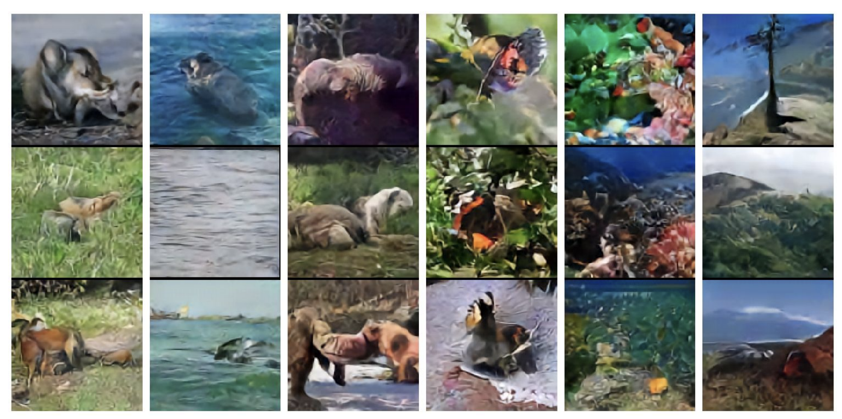
### Problems with VAEs
A common drawback of VAEs is that their generated images often appear blurry. The blurriness in VAE-generated images is largely due to the information bottleneck imposed by the latent variable $ z $. Since $ z $ is sampled from a low-dimensional distribution (e.g., $ \mathcal{N}(0, I) $) and must encode all the information needed to reconstruct $ x $, the model may struggle to retain fine details. The decoder then fills in missing information by producing the average of likely reconstructions, resulting in blurry outputs. This is especially problematic when the latent space is too constrained or when the model is uncertain.
In contrast, GANs (Generative Adversarial Networks) directly learn to generate sharp images by training against a discriminator that penalizes unrealistic outputs. Unlike VAEs, GANs do not explicitly model likelihoods or pixel-level uncertainty, which allows them to generate crisper images but at the cost of less interpretable latent spaces.
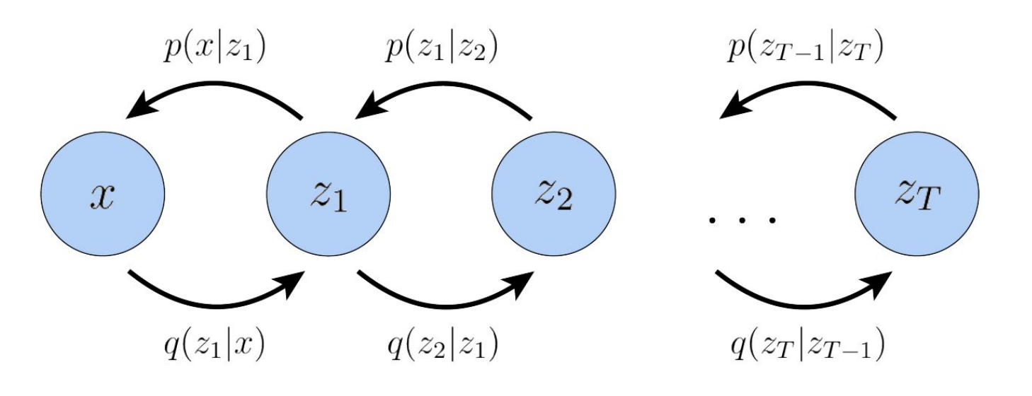
## Hierarchial VAEs
Hierarchical VAEs extend the basic VAE architecture by introducing multiple layers of latent variables, forming a hierarchy. Instead of modeling the data using a single latent variable $ z $, the generative process is defined as a Markov chain: each latent variable $ z_t $ is generated conditionally from the one above it, $ z_{t+1} $. This structure allows the model to capture complex dependencies and multi-scale representations—higher layers can encode more abstract, global features, while lower layers focus on finer details.
Formally, the generative model is:
$$
p(x, z_1, \dots, z_T) = p(x \mid z_1) p(z_1 \mid z_2) \cdots p(z_{T-1} \mid z_T) p(z_T)
$$
And the inference model (encoder) mirrors this structure:
$$
q(z_T \mid z_{T-1}) \cdots q(z_2 \mid z_1) q(z_1 \mid x)
$$
This hierarchical approach improves the expressiveness of the latent space, allowing better generation and more structured representations than a single-layer VAE.
## Summary
* Generative image models aim to map samples from a standard normal Gaussian distribution to the image manifold.
* GANs learn this mapping using a discriminator to distinguish real from generated images.
* VAEs learn it by optimizing a variational objective that encourages reconstruction and regularization.
* Autoencoders are designed to compress data into a latent space and reconstruct it from that space.
* VAEs extend autoencoders by making them probabilistic, allowing the model to sample from distributions rather than fixed encodings.
* The reconstruction loss encourages the decoder to produce outputs close to the original input.
* The latent variables are sampled from Gaussian distributions, introducing uncertainty into the encoding process.
* The reparameterization trick allows gradients to flow through the sampling operation, enabling end-to-end training.
* The KL divergence penalizes deviation from the standard normal prior, regularizing the latent space.
* The ELBO (Evidence Lower Bound) is optimized as a proxy for the true data likelihood.
* Maximizing the ELBO and minimizing the KL divergence pushes $ P(x \mid z) $ to closely approximate the true data distribution $ P(x) $.