# Diffusion 1: Introduction to Diffusion Models
## Background And Motivation
Image generation via artificial intelligence has been around for quite some time. **Deep Generative Models** refers to a class of models leverage deep learning to learn and sample from complex data distributions, such as those of natural images.
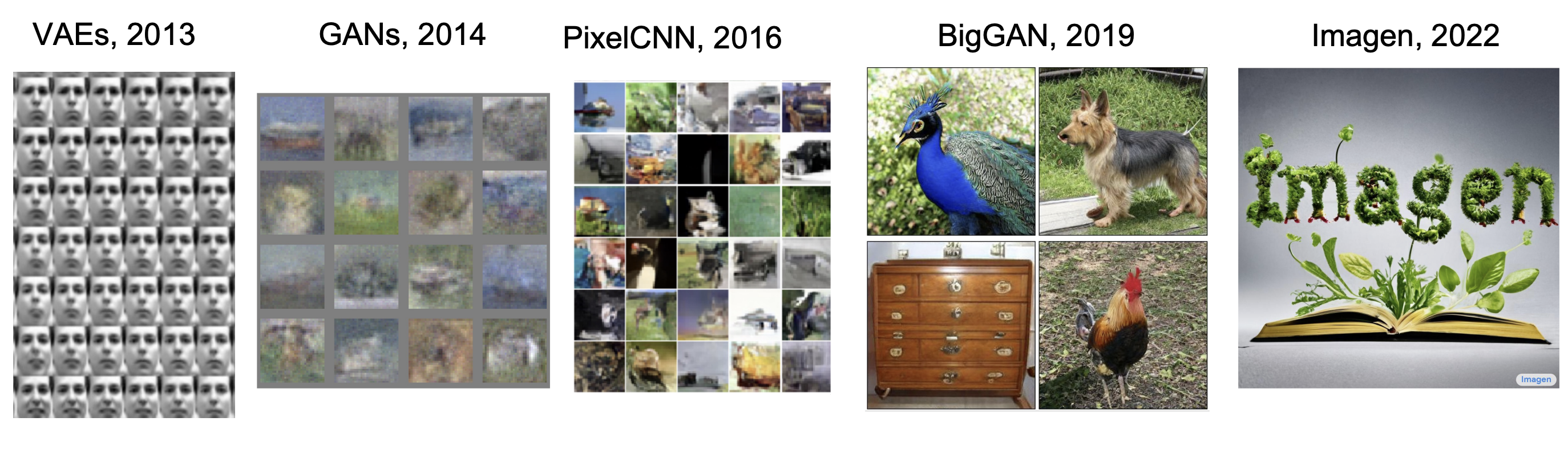
Several prominent architectures have shaped the trajectory of deep generative modeling:
[Cornell University, 2025, *CS 4782: Week 9 Lecture Slides*]
1. Variational Autoencoders were some of the first models to produce images of reasonable quality by learning a latent distribution, but they sufferred from bluriness due to the likelihood-based objective.
2. GANs succeeded them by replacing the likelihood objective with a minimax objective that generates sharper images, albeit with a more unstable training and suffering from mode collapse.
3. PixelCNN attempted to use an autoregressive approach to predict subsequent pixels, conditioned on the previous ones, but this suffered from slow training times due to the sequential computations.
4. BigGAN is a larger GAN model trained on datasets like ImageNet and created state-of-the-art images, but it still had training instability.
In 2022, Google introduced Imagen, a text-to-image diffusion model that combines the power of large language models (like T5) with a **diffusion-based** image generator. Imagen exemplifies **cross-modal** generation, where textual input is embedded and used to guide image synthesis.
This first set of notes, *Diffusion I*, focuses on the fundamentals of diffusion models through the lens of Denoising Diffusion Probabilistic Models (DDPMs) — covering their motivations, forward and reverse processes, and training objectives. Diffusion II will explore the conditioning process, score-based models, and extensions.
### Setting
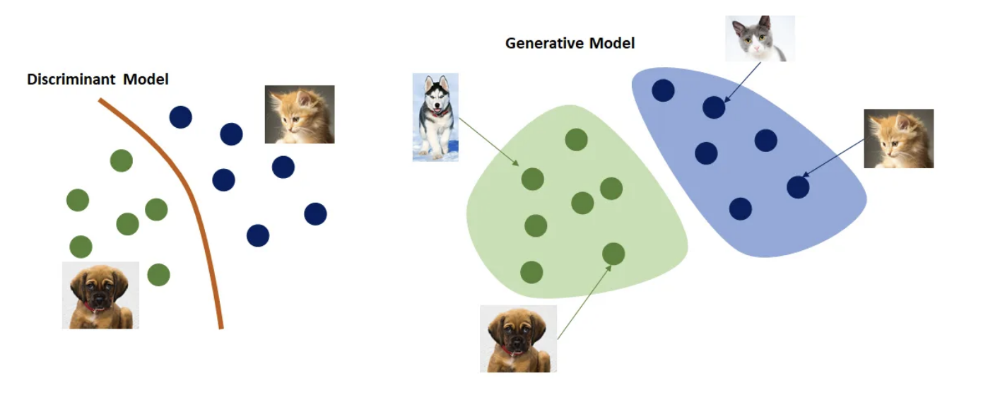
Let us recall the setting for image generation. Suppose we have some dataset $ \mathcal{D} = \{(x, y)\}_1^N $. As opposed to modeling a **decision boundary** as in discriminative learning, i.e. modeling the *distribution* $ P(y \mid x) $, we are instead modeling **how** the data is generated, i.e. the *distribution* $ P(x) $ directly.
[Esteve, 2018, *Step-by-step visual introduction to diffusion models*]
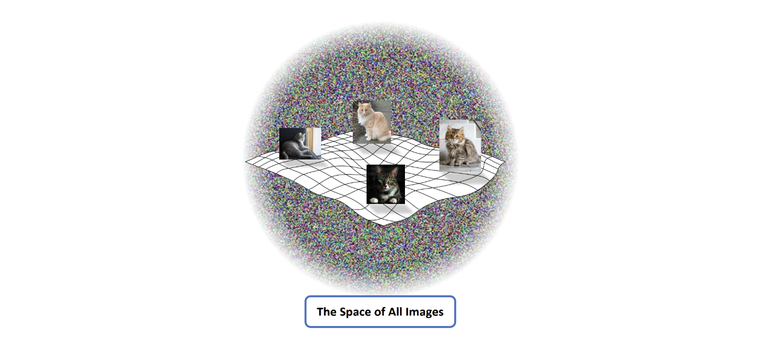
We are trying to generate images. But what does the **distribution** $ P(x) $ actually look like?
> 💡 **Observation:** If we think about the space of all images, we note that:
>
> 1. We have pictures of objects that humans can recognize (e.g. a chair, a table, etc.)
> 2. We have different transformations we can apply to them (inversions, rotations, translations, etc.), as well as combinations of objects.
> 3. But, these are all really just very **special cases** of random pixel configurations.
So the space of images is practically infinite. In fact, the **vast majority** of image configurations correspond to **meaningless noise**.
[Cornell University, 2020, *Training and GANs – Part 2*]
So one particular category of images, let's say cats, occupies an infintesimely small portion of this entire space. It actually forms what is called a low-dimensional **manifold**, which is a curved (nonlinear) generalization of a surface.
Learning this manifold $ P(x) $ is what makes AI image generation tricky!
> :brain: **Intuition:** Imagine putting together random pixels. What are the chances it looks like a cat? Basically zero!
## Introduction
So what **are** diffusion models?
Diffusion models are a class of generative models that learn to generate data by reversing a gradual noising process. The core idea is simple, yet powerful: take a clean image, and slowly corrupt it by adding small amounts of noise over many time steps — until it becomes nearly pure noise. Then, train a neural network to reverse this process, denoising step-by-step until the image is fully restored. This denoising process is learned using a parameterized model.
> 💡 **Observation:** By iteratively applying this reverse process starting from random noise, the model learns to synthesize new, realistic samples from scratch.
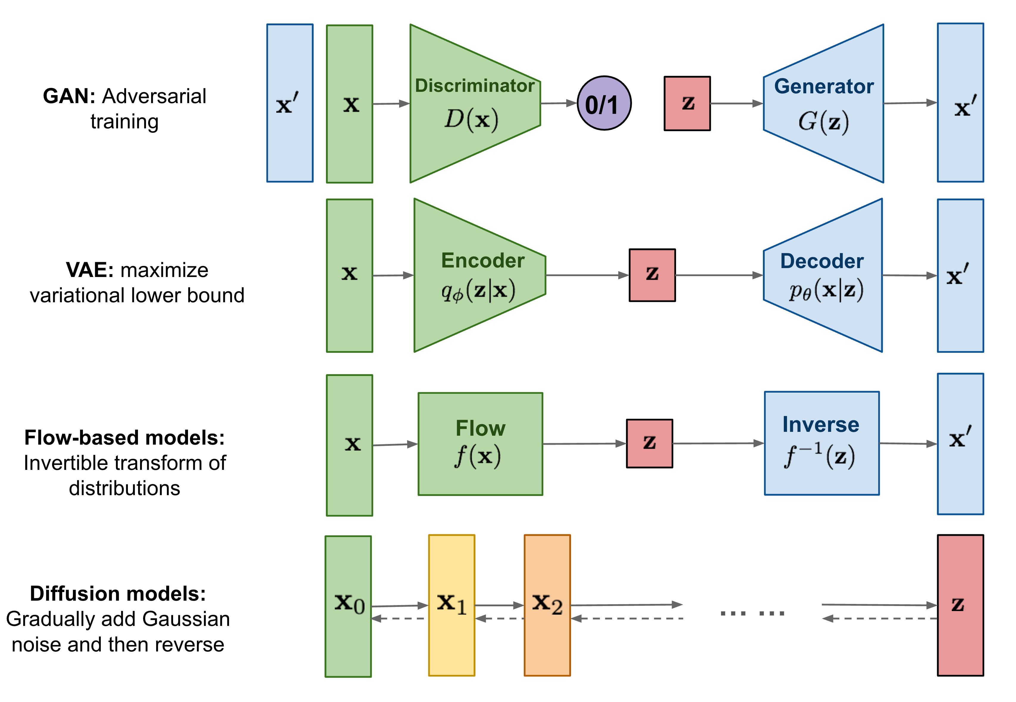
At a high level, diffusion models consist of two main components:
1. **Forward process (noising)**: A fixed, usually Gaussian, process that gradually destroys structure in the data by adding noise.
2. **Reverse process (denoising)**: A learned, probabilistic process that attempts to undo this destruction and reconstruct a data sample.
[Weng, 2021, *What are Diffusion Models?*]
Unlike GANs, diffusion models are trained with a stable likelihood-based objective, and unlike VAEs, they are capable of generating sharp, high-quality samples. In fact, modern diffusion models **outperform** GANs in both visual quality and diversity, as measured by metrics like FID.
In the next sections, we’ll break down how diffusion works — starting with the forward noising process and moving on to the reverse denoising and training objectives.
## The Forward Process (Noising)
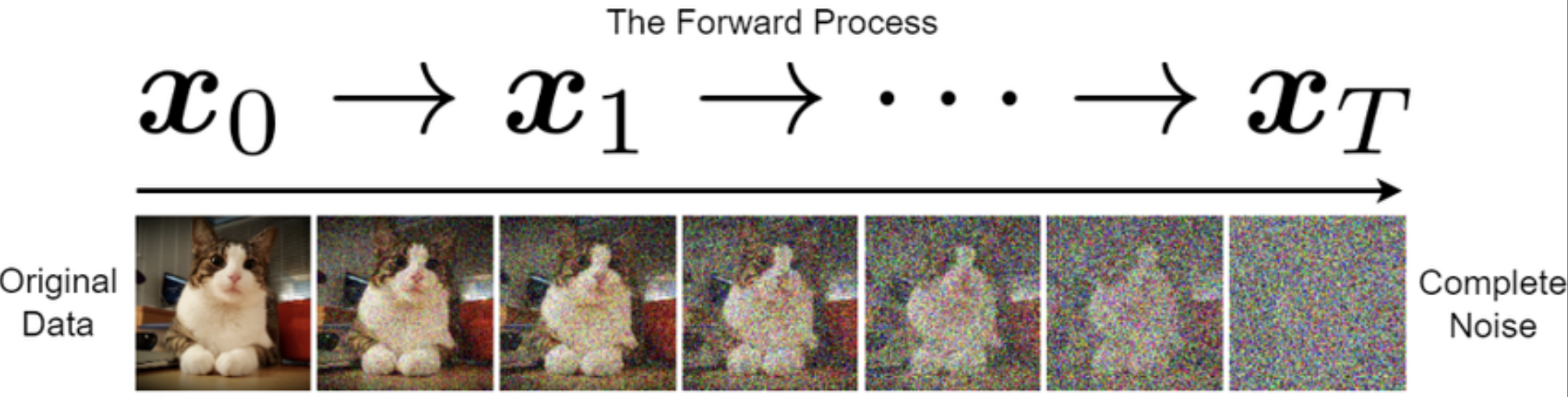
Let’s start with a cat 🐱.
Imagine we take an image of a cat and start adding a little bit of random Gaussian noise to it — just enough that it's still recognizable. Now imagine doing this over and over, for **hundreds** of steps, each time adding just a touch more noise. Eventually, the image becomes indistinguishable from pure static. This is the **forward diffusion process**.
[CVPR, 2022, *Diffusion Models*]
The goal of this process is to gradually transform a clean image $ x_0 $ into a noisy version $ x_T $ that is nearly standard Gaussian noise. Importantly, this process $ q $ is **fixed** and does not involve any learning — it defines a known corruption trajectory from data to noise.
[Cornell University, 2025, *CS 4782: Week 9 Lecture Slides*]
#### Some Math
We define a Markov chain of latent variables $ x_1, x_2, \ldots, x_T $ such that:
$$
q(x_{1:T} \mid x_0) = \prod_{t=1}^T q(x_t \mid x_{t-1})
$$
Each step adds Gaussian noise to the image:
$$
q(x_t \mid x_{t-1}) = \mathcal{N}(x_t; \sqrt{1 - \beta_t} \, x_{t-1}, \beta_t \, I)
$$
Here, $ \beta_t $ is a small positive number controlling how much noise we add at time step $ t $ — this sequence $ \{\beta_t\}_{t=1}^T $ is called the **noise schedule**.
Rather than sampling each $ x_t $ sequentially, we can jump directly from $ x_0 $ to any $ x_t $ using the closed-form:
$$
q(x_t \mid x_0) = \mathcal{N}(x_t; \sqrt{\bar{\alpha}_t} \, x_0, (1 - \bar{\alpha}_t) \, I)
$$
where $ \bar{\alpha}_t = \prod_{s=1}^t (1 - \beta_s) $.
> 💡 **Observation:** This means we can sample noisy versions of an image at any timestep $ t $ directly, without stepping through all intermediate states.
Let's derive this! First, we make the change of variable $ \alpha_t = 1 - \beta_t $ so that $ q(x_t \mid x_{t - 1}) = \mathcal{N}(x_t; \sqrt{\alpha_t}x_{t - 1}, (1 - \alpha_t)I) $. ❗️ This is just to make the math cleaner.
Now, recall the "reparameterization trick" for sampling from an arbitrary distribution. Namely, to sample $ x_t \sim q(x_t \mid x_{t - 1}) $, we let $ x_t = \sqrt{\alpha_t}x_{t - 1} + \sqrt{1 - \alpha_t}\epsilon $, where $ \epsilon \sim \mathcal{N}(0, 1) $. Let's use this to sample $ x_1 $ and $ x_2 $!
$$
\begin{align}
x_1 & = \sqrt{\alpha_1}x_0 + \sqrt{1 - \alpha_1}\epsilon_0 \tag{$ \epsilon_0 \sim \mathcal{N}(0, 1) $} \\
x_2 & = \sqrt{\alpha_2}x_1 + \sqrt{1 - \alpha_2}\epsilon_1 \tag{$ \epsilon_1 \sim \mathcal{N}(0, 1) $} \\
\to x_2 & = \sqrt{\alpha_2}\left(\sqrt{\alpha_1}x_0 + \sqrt{1 - \alpha_1}\epsilon_0\right) + \sqrt{1 - \alpha_2}\epsilon_1 \\
& = \sqrt{\alpha_1\alpha_2}x_0 + \sqrt{\alpha_2 - \alpha_1\alpha_2}\epsilon_0 + \sqrt{1 - \alpha_2}\epsilon_1
\end{align}
$$
Recall that for $ X, Y \sim \mathcal{N}(0, 1) $, $ Z = aX + bY \to Z \sim \mathcal{N}(0, a^2 + b^2) $. Let's use this to combine our noise by letting $ a = \sqrt{\alpha_2 - \alpha_1\alpha_2} $, $ b = \sqrt{1 - \alpha_2} $, and sampling $ z = 0 + \sqrt{a^2 + b^2}\epsilon $ where $ \epsilon \sim \mathcal{N}(0, 1) $:
$$
\begin{align}
\sqrt{\alpha_1\alpha_2}x_0 + \sqrt{\alpha_2 - \alpha_1\alpha_2}\epsilon_0 + \sqrt{1 - \alpha_2}\epsilon_1 & = \sqrt{\alpha_1\alpha_2}x_0 + \left(0 + \sqrt{\alpha_2 - \alpha_1\alpha_2 + 1 - \alpha_2}\epsilon\right) \tag{$ \epsilon \sim \mathcal{N}(0, 1) $} \\
& = \sqrt{\alpha_1\alpha_2}x_0 + \sqrt{1 - \alpha_1\alpha_2}\epsilon
\end{align}
$$
Passing this recursively until timestep $ t $, we get that
$$
\begin{align}
x_t & = \sqrt{\alpha_1\alpha_2 \cdots \alpha_t}x_0 + \sqrt{1 - \alpha_1\alpha_2 \cdots \alpha_t}\epsilon \tag{$ \epsilon \sim \mathcal{N}(0, 1) $} \\
& = \sqrt{\bar{\alpha}_t}x_0 + \sqrt{1 - \bar{\alpha}_t}\epsilon \tag{Let $ \bar{\alpha}_t = \alpha_1\alpha_2 \cdots \alpha_t $}
\end{align}
$$
From our reparameterization trick, we see that $ q(x_t \mid x_0) = \mathcal{N}(\sqrt{\bar{\alpha}_t}x_0, (1 - \bar{\alpha}_t)I) $. 💡 Note that the mean is **dependent** on $ x_0 $. This will become relevant later!
#### Why Do This?
The reason for all this noise is to **map the data distribution to something simple** — ideally, standard Gaussian noise. Once the data is fully corrupted, we can then learn how to **reverse** the process, step by step, and recover a realistic sample. This setup allows us to frame generation as learning to reverse a known stochastic process.
In the next section, we’ll look at how to learn the reverse denoising process, and how it allows us to sample new images by running this process backward from pure noise.
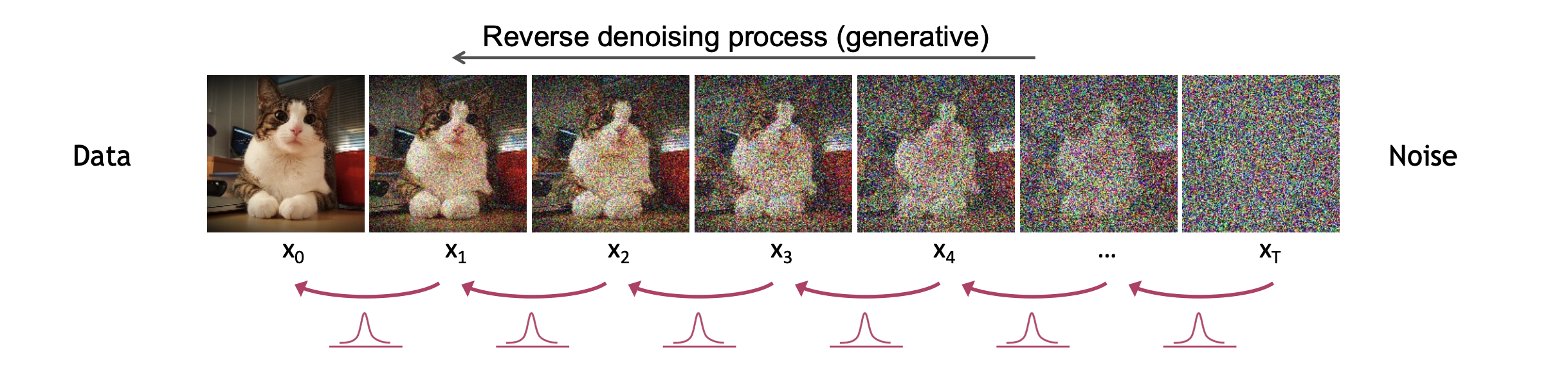
## The Reverse Process (Denoising)
Now that we have a noised image, it is time to denoise! We seek to find an $ x_0 $ which was on the original data manifold.
[CVPR, 2022, *Diffusion Models*]
As you can see, we are coming from our Gaussian noise $ p(x_T) $ and we want to gradually denoise all the way back to our original manifold.
> ⚠️ **Warning:** In practice, $ T $ is typically **very** large. So this process is actually quite *computationally intensive*.
##### But Why Not Just Denoise in One Step, vis. GANs?
One of the biggest advantages of GANs are their generation speed! But this comes at its own cost:
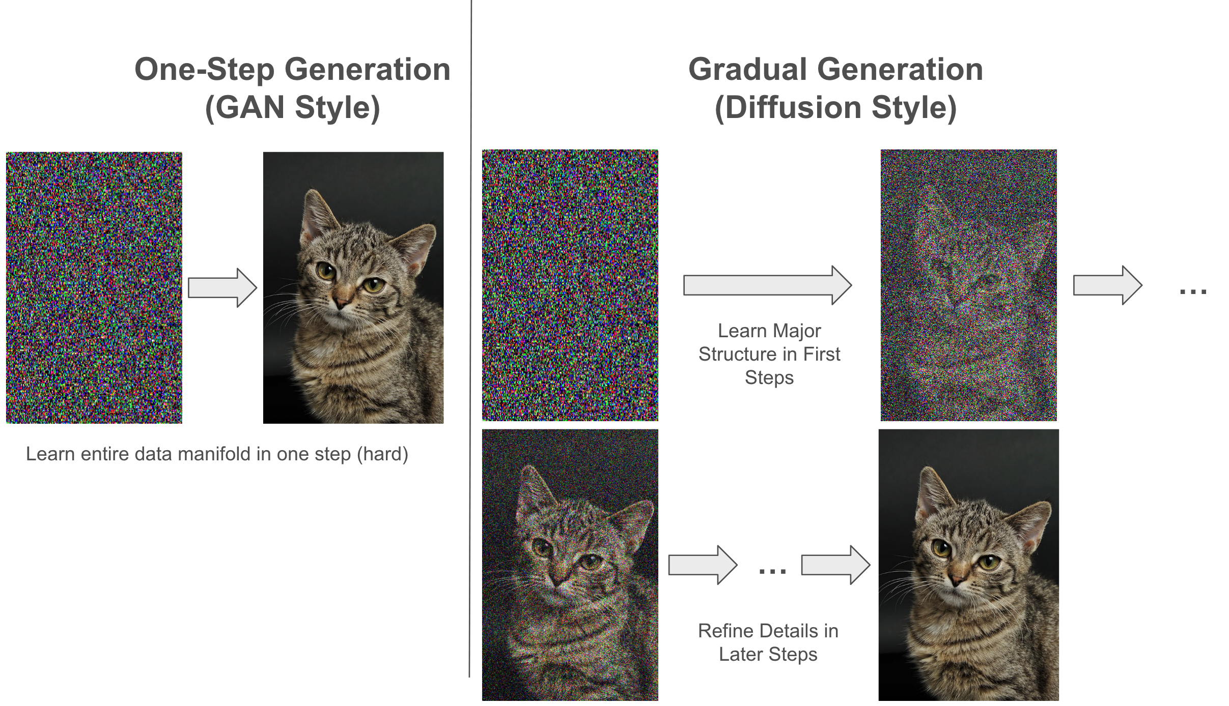
❗️Both Diffusion and GANs **can** generate high quality images. But given an arbitrary noise image, GANs have to learn the *entire* image manifold in just **one time step**. Even just conceptualizing that task makes it seem unviable! And this is precisely what leads to GANs having mode collapse:
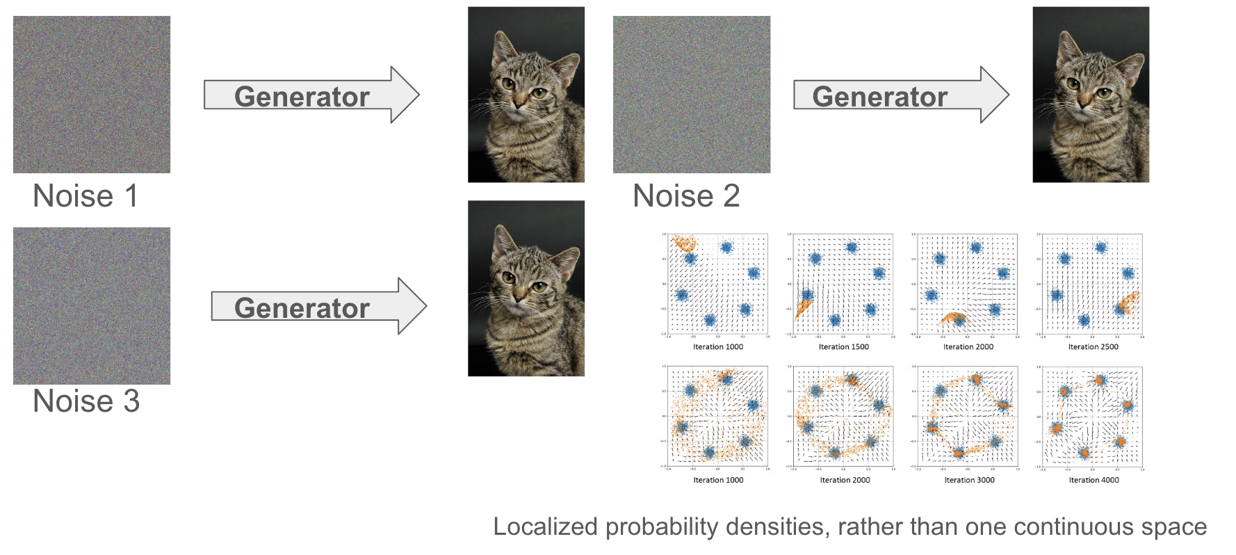[Gainetinov, 2024, *Understanding GAN Mode Collapse: Causes and Solutions*]
Unrelated Gaussian noise images are denoising to the exact same target image! We are experiencing *mode collapse*. It turns out that denoising in one time step just isn't **expressive** enough, and we need more complexity! Diffusion is able to get around this by:
1. ⛰ Learning high-level, *structural* details of the manifold in early time steps
2. 👁 Refining for image quality and detail at later time steps
> ⚠️ **Warning:** Our choice of *noise schedule* matters a lot here! Linear scheduling (upper row) requires more time steps, and it seems you already lost all your information at the halfway point. Cosine scheduling (bottom row) in this case can be more gradual, and decreases time steps from 1000 to only 50.


[Erdem, 2022, *Step-by-step visual introduction to diffusion models*]
### An Intractable Distribution
In the forward process, we add noise **stochastically** at each step, meaning there isn't a one-to-one mapping from input images to noisy outputs. Still, given an image \($ x_0 $\), we can compute the **distribution** of its noisy counterpart \($ x_t $\) in closed form — even though the actual sample \($ x_t $\) is random.
How do we reverse this process? Let's start by thinking about reversing just one time step.
##### Reversing One Timestep
Suppose we knew the distribution $ q(x_{t - 1} \mid x_t) $ . Then, we could take out $ x_t $ for $ t \in \{1, 2, \dots, T\} $ and sample an $ x_{t - 1} $, repeating the process. Let's try computing $ q(x_{t - 1} \mid x_t) $. First, let's recall Bayes' Rule for random variables $ A, B $:
$$
P(A \mid B) = \frac{P(B \mid A)P(A)}{P(B)}
$$
We apply this:
$$
\begin{align}
q(x_{t - 1} \mid x_t) & = \frac{q(x_t \mid x_{t - 1}) q(x_{t - 1})}{q(x_t)} \\
\end{align}
$$
We have already established that $ q(x_t \mid x_{t - 1}) \sim \mathcal{N}(\sqrt{\bar{\alpha}}x_0, (1 - \bar{\alpha})I) $. But what about $ q(x_{t - 1}) $ and $ q(x_t) $?
Recall the following facts from probability for continuous random variables $ A, B $ with joint pdf $ p(A, B) $:
$$
p(A) = \int p(A, B)dB \tag {Obtaining the marginal pdf of $ A, B $} \\
p(B) = \int p(A, B)dA \\
$$
$$
p(A, B) = p(A \mid B)p(B) \tag{Chain rule of probability}
$$
Can this help us here? We make the following attempt:
$$
\begin{align}
q(x_{t - 1}) & = \int \dots \int q(x_{t - 1}, x_{t - 2}, \dots, x_{0})dx_{t - 2}\dots dx_0 \tag{Marginalizing joint pdf} \\
& = \int q(x_{t - 1} \mid x_{t - 2})q(x_{t - 2} \mid x_{t - 3}) \dots q(x_1 \mid x_0)q(x_0) dx_{t - 2}\dots dx_0 \tag{Chain rule of probability}
\end{align}
$$
Notice the problem? We need $ q(x_0) $, which requires knowing the original data manifold! If we knew this, we would not be doing diffusion in the first place and would rather just sample from this manifold.
##### A Visualization 🖼
Let's step back. Suppose someone threw a ball, and the ball is now in mid air:
Take a look at the left side. If someone told you to calculate the probability that the ball was in that position in the air, you wouldn't be able to do it! That is an intractable computation, there are too many possibilities to consider. But what if we have more information? ❗️Aha! The right side tells us exactly where the ball came from. If we *condition* on this, our calculation is **much** simpler, but is it in fact tractable?
#### From Intractable to Tractable
Let us recall our setting. We noised an image $ x_0 $ sampled from the manifold deterministically using some noise schedule $ \{\bar{\alpha_t}\}_{t = 0}^T $ so that $ q(x_T) \approx \mathcal{N}(0, I) $. What if instead, we try to compute $ q(x_{t - 1} \mid x_t, x_0) $. That is, we condition on our initial image sample. Let's try this:
$$
\begin{align}
q(x_{t - 1} \mid x_t, x_0) & = \frac{q(x_{t - 1}, x_t, x_0)}{q(x_t, x_0)} \tag{Conditional rules} \\
& = \frac{q(x_t \mid x_{t - 1}, x_0)q(x_{t - 1} \mid x_0)q(x_0)}{q(x_t \mid x_0)q(x_0)} \tag{Chain rule of probability} \\
& = \frac{q(x_t \mid x_{t - 1}, x_0)q(x_{t - 1} \mid x_0)}{q(x_t \mid x_0)} \tag{Simplifying} \\
& = \frac{q(x_t \mid x_{t - 1})q(x_{t - 1} \mid x_0)}{q(x_t \mid x_0)} \tag{Markovian Assumption}
\end{align}
$$
> 📝**Note:** In the last step, we applied the Markovian Assumption, namely that given the present $ x_{t - 1} $, the *future* $ x_t $ is **independent** of the *past* (i.e. $ x_0 $ ).
Now, is this tractable? Recall that $ q(x_t \mid x_0) \sim \mathcal{N}(\sqrt{\bar{\alpha}_t}x_0, (1 - \bar{\alpha}_t)I) $ and $ q(x_{t - 1} \mid x_0) \sim \mathcal{N}(\sqrt{\bar{\alpha}_{t - 1}}x_0, (1 - \bar{\alpha}_{t - 1})I) $ as we derived this for a general timestep $ t $. Also, $ q(x_t \mid x_{t - 1}) \sim \mathcal{N}(\sqrt{1 - \beta_t}x_{t - 1}, \beta_tI) $, which was our original noising formulation for one timestep. So, this is entirely tractable! But there remains a problem.
## Architecture of the Denoising Model
So far, we've focused on what the model learns. Now let's briefly discuss **how** it's implemented.
The function $ \epsilon_\theta(x_t, t) $ is modeled using a neural network that takes in a noised image \( x_t \) and a timestep \( t \), and outputs an estimate of the noise. The most common architecture is a **U-Net**, originally used for segmentation tasks, but adapted for diffusion by:
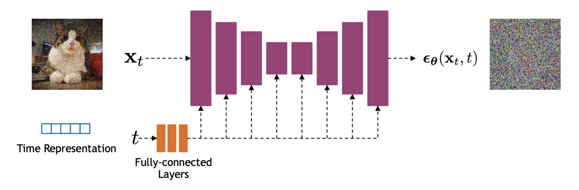
[Cornell University, 2025, *CS 4782: Week 9 Lecture Slides*]
- Using **residual blocks** for stable training
- Adding **skip connections** to preserve spatial detail
- Including **self-attention** layers to capture long-range dependencies
- Injecting **sinusoidal positional encodings** for the timestep \( t \), which are added or concatenated throughout the network
The output of this model has the same shape as the input image. It can be trained to predict:
- The original image $ x_0 $
- The mean $ \mu_q $
- Or, most commonly, the noise $ \epsilon_0 $ used to generate $ x_t $
Modern variants like *Imagen*, *Latent Diffusion*, and *ControlNet* all build on this U-Net backbone with enhancements (e.g., attention over text embeddings, cross-conditioning, or latent-space modeling).
> 💡 **Observation:** Because the same model must denoise across all timesteps \( t \), it must generalize across a wide range of signal-to-noise ratios, making time conditioning and expressive capacity crucial.
### What About During Inference?
We originally were trying to compute $ q(x_{t - 1} \mid x_t) $. If we had this, we could just denoise deterministically by sampling from this distribution. But, to make this tractable, we relaxed this to compute intstead $ q(x_{ t - 1} \mid x_t, x_0) $. **This requires knowing the original image we noised from**. If we are trying to sample a Gaussian noise vector $ x_T $ and denoise to an image on our manifold, we *canno*t do this! So, we will need a strategy to combat this.
#### A Generative Model $ p_\theta $
What if we combine these two approaches? We use $ q(x_{t - 1} \mid x_t, x_0) $ to learn some $ p_\theta(x_{t - 1} \mid x_t) $ that is independent of $ x_0 $. This would allows us to denoise during inference time **without knowledge of $ x_0 $!** Recall that we can use neural networks to learn the parameters $ \theta $ of a distribution, so we parameterize our distribution as $ p_\theta(x_{t - 1} \mid x_t) $. For example, in VAEs, we learned $ \mu $ and $ \log(\sigma^2) $ of our distribution that encodes to the latent space. We are doing something very similar here!
At time step $ t $, we are lost at foggy (noised) landscape, unsure of how to get back to our original manifold. We use $ p_\theta $ to *guide* us back one time step and suddenly we can see a road to take which will ultimately lead us back to an image on the original manifold, $ x_0 $!
#### Constructing An Objective
So we are trying to learn some distribution parameterized by $ \theta $ so that $ p_\theta(x_{t - 1} \mid x_t) $ resembles our tractable distribution $ q(x_{t - 1} \mid x_t, x_0) $. How can we accomplish this? Recall the KL Divergence between distributions $ p, q $:
$$
D_{\rm{KL}}(p || q) = \mathbb{E}_{x \sim p}\left[\log \frac{p(x)}{q(x)}\right]
$$
We can apply this with our distributions! But, recall that KL divergence is not symmetric. So our choice of which distribution to use as $ p $ and which to use as $ q $ matters here. The KL divergence measured how much information is lost when you use $ q $ to approximate $ p $. Since we are using $ p_\theta(x_{t - 1} \mid x_t) $ as an approximator, it makes sense to use it in place of $ q $. So, we can have the fully tractable term:
$$
\begin{align}
\mathbb{E}_{q(x_t \mid x_0)}\left[D_{KL} \left(q\left(x_{t - 1} \mid x_t, x_0) || p_{\theta}(x_{t - 1} \mid x_t\right)\right)\right]
\end{align}
$$
Recall our ELBO from the VAEs lecture:
$$
\begin{align}
\log p(x) & \geq \mathbb{E}_{q_\phi(z \mid x)} \left[\log p_\theta\left(x \mid z\right)\right] - D_{KL}\left(q_\phi\left(z \mid x\right) || p\left(z\right)\right)
\end{align}
$$
We observe the following:
1. We call the first term the **reconstruction** term because we are reconstructing an $ x $ on our original manifold from the latent $ z $
2. The second term is the **prior** matching term because we want our latent $ z $'s distribution to match the Unit Gaussian prior
##### Terms for Diffusion ELBO
What are our **diffusion analogs** here? We only get an original $ x $ on the manifold once we denoise from $ x_1 $. Likewise, we want to make sure that when we noise all the way to our last time step $ T $, we get a Unit Gaussian distribution. So intuitively, our corresponding terms are:
1. Reconstruction: $ \mathbb{E}_{q(x_1 \mid x_0)} \left[\log p_\theta \left(x_0 \mid x_1\right)\right] $
2. $ D_{KL}\left(q\left(x_T \mid x_0\right) || p\left(x_T\right)\right) $
So this leaves us with the following objective:
$$
\begin{align}
\mathbb{E}_{q(x_1 \mid x_0)} \left[\log p_\theta (x_0 \mid x_1)\right] - D_{KL}\left(q(x_T \mid x_0) || p(x_T)\right) + \sum_{t = 2}^T + \mathbb{E}_{q(x_t \mid x_0)} \left[D_{KL} \left(q(x_{t - 1} \mid x_t, x_0) || p_{\theta}(x_{t - 1} \mid x_t)\right)\right]
\end{align}
$$
> 📝 **Note:** The reconstruction term is actually independent of $ \theta $, so it does not contribute to the gradient flow for training our generative model $ p_\theta $. This term is actually only relevant in the forward noising process.
#### Deriving The ELBO
But does this objective actually mean anything? In particular, does optimizing it ensure we denoise to data close to our original data manifold? In fact, yes it does. The log likelihood lower bound derivation is as follows:
$$
\begin{align}
\log p(x) & = \log \int p(x_{0:T}) dx_{1:T} \tag{Marginalizing joint pdf} \\
& = \log \int \frac{p(x_{0:T})q(x_{1:T} \mid x_0)}{q(x_{1:T} \mid x_0)} \tag{Multiply by $ 1 $} \\
& = \log \mathbb{E}_{q(x_{1:T} \mid x_0)} \left[\frac{p(x_{0:T})}{q(x_{1:T} \mid x_0)}\right] \tag{Definition of expectation} \\
& \geq \mathbb{E}_{q(x_{1:T} \mid x_0)} \left[\log \frac{p(x_{0:T})}{q(x_{1:T} \mid x_0)}\right] \tag{Jensen's Inequality} \\
& = \mathbb{E}_{q(x_{1:T} \mid x_0)} \left[\log \frac{p(x_T) \prod_{t = 1}^T p_\theta(x_{t - 1} \mid x_t)}{\prod_{t = 1}^T q(x_t \mid x_{t - 1})}\right] \tag{Chain rule of probability} \\
& = \mathbb{E}_{q(x_{1:T} \mid x_0)} \left[\log \frac{p(x_T)p_\theta(x_0 \mid x_1) \prod_{t = 2}^T p_\theta(x_{t - 1} \mid x_t)}{q(x_1 \mid x_0)\prod_{t = 2}^{T} q(x_t \mid x_{t - 1})}\right] \\
& = \mathbb{E}_{q(x_{1:T} \mid x_0)} \left[\log \frac{p(x_T)p_\theta(x_0 \mid x_1) \prod_{t = 2}^T p_\theta(x_{t - 1} \mid x_t)}{q(x_1 \mid x_0)\prod_{t = 2}^{T} q(x_t \mid x_{t - 1}, x_0)}\right] \tag{Markovian Assumption} \\
& = \mathbb{E}_{q(x_{1:T} \mid x_0)} \left[\log \frac{p(x_T)p_\theta(x_0 \mid x_1) \prod_{t = 2}^T p_\theta(x_{t - 1} \mid x_t)}{q(x_1 \mid x_0)\prod_{t = 2}^{T} \frac{q(x_{t - 1} \mid x_t, x_0)q(x_t \mid x_0)}{q(x_{t - 1} \mid x_0)}}\right] \tag{Bayes' Rule} \\
& = \mathbb{E}_{q(x_{1:T} \mid x_0)} \left[\log \frac{p(x_T)p_\theta(x_0 \mid x_1) \prod_{t = 2}^T p_\theta(x_{t - 1} \mid x_t)}{q(x_1 \mid x_0) \frac{q(x_T \mid x_0)}{q(x_1 \mid x_0)} \frac{\prod_{t = 2}^{T - 1} q(x_t \mid x_0)}{\prod_{t = 3}^{T} q(x_{t - 1} \mid x_0)}\prod_{t = 2}^{T} q(x_{t - 1} \mid x_t, x_0)}\right] \\
& = \mathbb{E}_{q(x_{1:T} \mid x_0)} \left[\log \frac{p(x_T)p_\theta(x_0 \mid x_1) \prod_{t = 2}^T p_\theta(x_{t - 1} \mid x_t)}{q(x_1 \mid x_0) \frac{q(x_T \mid x_0)}{q(x_1 \mid x_0)} \frac{\prod_{t = 2}^{T - 1} q(x_t \mid x_0)}{\prod_{t = 2}^{T - 1} q(x_{t} \mid x_0)} \prod_{t = 2}^{T} q(x_{t - 1} \mid x_t, x_0)}\right] \tag{Re-indexing} \\
& = \mathbb{E}_{q(x_{1:T} \mid x_0)} \left[\log \frac{p(x_T)p_\theta(x_0 \mid x_1) \prod_{t = 2}^T p_\theta(x_{t - 1} \mid x_t)}{q(x_T \mid x_0) \prod_{t = 2}^{T} q(x_{t - 1} \mid x_t, x_0)}\right] \tag{Simplifying} \\
& = \mathbb{E}_{q(x_{1:T} \mid x_0)} \left[\log \frac{p(x_T)p_\theta(x_0 \mid x_1)}{q(x_T \mid x_0)}\right] + \mathbb{E}_{q(x_{1:T} \mid x_0)} \left[\log \prod_{t = 2}^{T} \frac{p_\theta(x_{t - 1} \mid x_{t})}{q(x_{t - 1} \mid x_t, x_0)}\right] \tag{Properties of logarithms} \\
& = \mathbb{E}_{q(x_{1} \mid x_0)} \left[p_\theta(x_0 \mid x_1)\right] - \mathbb{E}_{q(x_{T} \mid x_0)} \left[\log \frac{q(x_T \mid x_0)}{p(x_T)}\right] - \sum_{t = 2}^{T} \mathbb{E}_{q(x_{t, t - 1} \mid x_0)} \left[\log \frac{q(x_{t - 1} \mid x_t, x_0)}{p_\theta(x_{t - 1} \mid x_{t})}\right] \tag{Simplifying expectation dependencies} \\
& = \underbrace{\mathbb{E}_{q(x_1 \mid x_0)} \left[\log p_\theta (x_0 \mid x_1)\right]}_{\rm{Reconstruction\ Term}} - \underbrace{D_{KL}\left(q(x_T \mid x_0) || p(x_T)\right)}_{\rm{Prior\ Matching\ Term}} + \underbrace{\sum_{t = 2}^T + \mathbb{E}_{q(x_t \mid x_0)} \left[D_{KL} \left(q(x_{t - 1} \mid x_t, x_0) || p_{\theta}(x_{t - 1} \mid x_t)\right)\right]}_{\rm{Denoising\ Matching\ Term}}
\end{align}
$$
[Ho, 2020, *Denoising diffusion probabilistic models*]
> ⚠️ **Warning:** The prove above relies on the Markovian assumption from the forward denoising process, so be sure to familiarize yourself with it and step through the proof to see where it is necessary as an exercise.
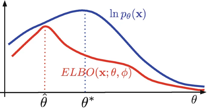
So what did we actually derive here? We have a lower bound on the log-likelihood of our data manifold $ p(x) $! So, as we optimize our lower bound, we will approach the true data manifold!
[Blei, 2021, *Variational inference: Foundations and methods*]
In particular, we **cannot** do any worse than the red line in the graphic, as this is a lower bound on our performance. The tighter we make this, the better results we expect!
### Revising Our Objective
Let's discuss what we are actually learning. We have some tractable posterior distribution $ q(x_{t - 1} \mid x_t, x_0) $. This is **Gaussian** because we already derived that $ q(x_{t - 1} \mid x_t, x_0) = \frac{q(x_t \mid x_{t - 1})q(x_{t - 1} \mid x_0)}{q(x_t \mid x_0)} $, and each of these terms is Gaussian.
> 📝 **Note:** To check your understanding, write out the distributions of each of these.
In fact, we note that:
$$
\begin{align}
q(x_{t - 1} \mid x_t, x_0) & = \frac{q(x_t \mid x_{t - 1})q(x_{t - 1} \mid x_0)}{q(x_t \mid x_0)} \\
& = \frac{\mathcal{N}(x_t; \sqrt{\alpha_t}x_{t - 1}, (1 - \alpha_t)I)\mathcal{N}(x_{t - 1}; \sqrt{\bar{\alpha}_{t - 1}}x_0, ( - \bar{\alpha}_{t - 1})I)}{\mathcal{N}(x_t; \sqrt{\bar{\alpha}_t}x_0, (1 - \bar{\alpha}_t)I)} \tag{Noising distributions} \\
& \propto \mathcal{N}(x_{t - 1}; \underbrace{\frac{\sqrt{\alpha_t}(1 - \bar{\alpha}_{t - 1})x_{t} + \sqrt{\bar{\alpha}_{t - 1}}(1 - \alpha_t)x_0}{1 - \bar{\alpha}_t}}_{\mu_q(x_t, x_0)}, \underbrace{\frac{(1 - \alpha_t)(1 - \bar{\alpha}_{t - 1})}{1 - \bar{\alpha_t}}}_{\Sigma_q(t)})
\end{align}
$$
📝 To see the full derivation of this, checkout [2]! Note that $ \mu_q $ depends both on $ x_t, x_0 $, whereas $ \Sigma_q $ is only dependent on $ t $, hence the parameterizations.
#### Mean Prediction Network
Hence, let's call our tractable distribution $ q(x_{t - 1} \mid x_t, x_0) \sim \mathcal{N}(x_{t - 1}; \mu_q; \Sigma_q(t)) $. We are learning the distribution $ p_\theta(x_{t - 1} \mid x_t) \sim \mathcal{N}(x_{t - 1}; \mu_\theta; \Sigma_q) $ . Why do we give each of these the *same* variance? Recall from the forward process that $ q(x_t \mid x_0) \sim \mathcal{N}(\sqrt{\bar{\alpha}_t}x_0, (1 - \bar{\alpha}_t I) $. So our variance at each timestep is independent of $ x_0 $! Hence, we can reuse it during inference. But, we have to *learn* the mean since that is dependent upon $ x_0 $.
Now, we simplify the following objective:
$$
\begin{align}
D_{KL}(q(x_{t - 1} \mid x_t, x_0) || p_\theta(x_{t - 1} | x_t)) & = D_{KL}(\mathcal{N}(x_{t - 1}; \mu_q; \Sigma_q(t)) || \mathcal{N}(x_{t - 1}; \mu_\theta; \Sigma_q(t))) \\
& = \frac{1}{2}\left[\log \frac{|\Sigma_q(t)|}{|\Sigma_q(t)|} - d + \rm{tr}\left(\Sigma_q(t)^{-1}\Sigma_q(t)\right) + \left(\mu_\theta - \mu_q\right)^\top \Sigma_q(t)^{-1} \left(\mu_\theta - \mu_q\right)\right] \tag{Formula for Gaussian KL Divergence} \\
& = \frac{1}{2}\left[\log(1) - d + d + \left(\mu_\theta - \mu_q\right)^\top \Sigma_q(t)^{-1} \left(\mu_\theta - \mu_q\right) \right] \\
& = \frac{1}{2}\left[\left(\mu_\theta - \mu_q\right)^\top \Sigma_q(t)^{-1} \left(\mu_\theta - \mu_q\right) \right] \\
& = \frac{1}{2}\left[\left(\mu_\theta - \mu_q\right)^\top (\sigma_q^2 I)^{-1} \left(\mu_\theta - \mu_q\right) \right] \tag{Covariance matrix} \\
& = \frac{1}{2\sigma_q^2}\left[\left(\mu_\theta - \mu_q\right)^\top\left(\mu_\theta - \mu_q\right) \right] \tag{Inverse of diagonal matrix} \\
& = \frac{1}{2\sigma_q^2}||\mu_\theta - \mu_q||_2^2 \tag{2-norm definition} \\
\end{align}
$$
Voila! We see that our denoising matching term objective is the same as the MSE between the two means.
#### Original Image Network
Now, what happens when we plug in our derivation (36) into this result?
$$
\begin{align}
D_{KL}(q(x_{t - 1} \mid x_t, x_0) || p_\theta(x_{t - 1} | x_t)) & = \frac{1}{2\sigma_q^2}||\mu_\theta - \mu_q||_2^2 \\
& = \frac{1}{2\sigma_q^2}||\frac{\sqrt{\alpha_t}(1 - \bar{\alpha}_{t - 1})x_{t} + \sqrt{\bar{\alpha}_{t - 1}}(1 - \alpha_t)\hat{x}_\theta(x_t, t)}{1 - \bar{\alpha}_t} - \frac{\sqrt{\alpha_t}(1 - \bar{\alpha}_{t - 1})x_{t} + \sqrt{\bar{\alpha}_{t - 1}}(1 - \alpha_t)x_0}{1 - \bar{\alpha}_t}||_2^2 \tag{$ \hat{x}_\theta(x_t, t) $ is a predictor NN for $ x_0 $} \\
& = \frac{1}{2\sigma_q^2}||\frac{\sqrt{\bar{\alpha}_{t - 1}}(1 - \alpha_t)\hat{x}_\theta(x_t, t)}{1 - \bar{\alpha}_t} - \frac{\sqrt{\bar{\alpha}_{t - 1}}(1 - \alpha_t)x_0}{1 - \bar{\alpha}_t}||_2^2 \\
& = \frac{1}{2\sigma_q^2}\frac{\bar{\alpha}_{t - 1}(1 - \alpha_t)^2}{(1 - \bar{\alpha}_t)^2}||\hat{x}_\theta(x_t, t) - x_0||_2^2
\end{align}
$$
So we can alternatively view our optimization problem as just learning a neural network for the original denoised image. Do we have any other options?
#### Noise Prediction Network
Recall how we sample from our distribution $ q(x_t \mid x_0) \sim \mathcal{N}(\sqrt{\bar{\alpha}_t}x_0, (1 - \bar{\alpha}_t)I) $. So, we get $ x_t = \sqrt{\bar{\alpha}_t}x_0 + \sqrt{1 - \bar{\alpha}_t}\epsilon_0 $ where $ \epsilon_0 \sim \mathcal{N}(0, 1) $. Rearranging this, we get $ x_0 = \frac{x_t - \sqrt{1 - \bar{\alpha}_t}\epsilon_0}{\sqrt{\bar{\alpha}_t}} $. Let's plug this into our derivation above!
$$
\begin{align}
D_{KL}(q(x_{t - 1} \mid x_t, x_0) || p_\theta(x_{t - 1} | x_t)) & = \frac{1}{2\sigma_q^2}\frac{\bar{\alpha}_{t - 1}(1 - \alpha_t)^2}{(1 - \bar{\alpha}_t)^2}||\hat{x}_\theta(x_t, t) - x_0||_2^2 \\
& = \frac{1}{2\sigma_q^2}\frac{\bar{\alpha}_{t - 1}(1 - \alpha_t)^2}{(1 - \bar{\alpha}_t)^2}||\frac{x_t - \sqrt{1 - \bar{\alpha}_t}\hat{\epsilon}_\theta(x_t, t)}{\sqrt{\bar{\alpha}_t}} - \frac{x_t - \sqrt{1 - \bar{\alpha}_t}\epsilon_0}{\sqrt{\bar{\alpha}_t}}||_2^2 \tag{$ \hat{\epsilon}_\theta(x_t, t) $ is a predictor NN for $ x_0 $} \\
& = \frac{1}{2\sigma_q^2}\frac{\bar{\alpha}_{t - 1}(1 - \alpha_t)^2}{(1 - \bar{\alpha}_t)^2}||\frac{\sqrt{1 - \bar{\alpha}_t}}{\sqrt{\bar{\alpha}_t}}(\epsilon_0 - \hat{\epsilon}_\theta(x_t, t)||_2^2 \tag{Simplifying} \\
& = \frac{1}{2\sigma_q^2}\frac{\bar{\alpha}_{t - 1}(1 - \alpha_t)^2}{\bar{\alpha}_t(1 - \bar{\alpha}_t)}||\epsilon_0 - \hat{\epsilon}_\theta(x_t, t)||_2^2 \\
& = \frac{1}{2\sigma_q^2}\frac{(1 - \alpha_t)^2}{\alpha_t(1 - \bar{\alpha}_t)}||\epsilon_0 - \hat{\epsilon}_\theta(x_t, t)||_2^2 \tag{$ \frac{\bar{\alpha}_{t - 1}}{\bar{\alpha}_t} = \frac{1}{\alpha_t} $}
\end{align}
$$
So, from out neural network $ \hat{\epsilon}_\theta(x_t, t) $ which predicts the noise $ \epsilon_0 $ that uniquely determines $ x_t $ from $ x_0 $.
> ⚠️ **Warning:** This is not the noise that takes $ x_{t - 1} $ to $ x_t $! This is actually a *very* important distinction because we already know from our noise schedule the exact noise given to $ x_{t - 1} $ to produce $ x_t $. This is just $ \beta_t $! So we would not need to learn this. But we also know that $ x_0 $ is noised with $ \bar{\alpha}_t $ to produce $ x_t $, so why do we need to learn this quantity instead? This again boils down to the very reason why we are doing any learning for diffusion in the first place. We **do not** know $ x_0 $ during inference time, so to generate new samples, we need to learn how to get back to the original data manifold by having many $ x_0 $ from which we learn.
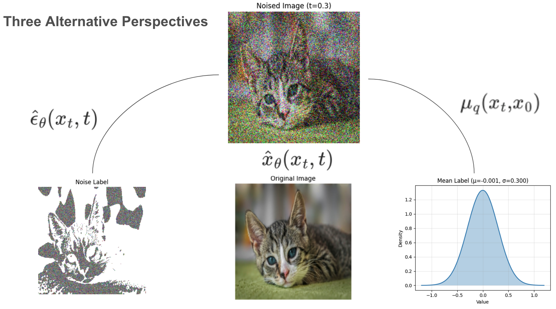
In the above visualization, you can see what each of these three networks are predicting, given some noised image $ x_t $ and timestep $ t $. These are three equivalent approaches.
#### Three (Somewhat) Equivalent Perspectives
We have all three perspectives now as follows:
$$
\begin{align}
D_{KL}(q(x_{t - 1} \mid x_t, x_0) || p_\theta(x_{t - 1} | x_t)) & = \frac{1}{2\sigma_q^2}||\mu_\theta - \mu_q||_2^2 \\
& = \frac{1}{2\sigma_q^2}\frac{\bar{\alpha}_{t - 1}(1 - \alpha_t)^2}{(1 - \bar{\alpha}_t)^2}||\hat{x}_\theta(x_t, t) - x_0||_2^2 \\
& = \underbrace{\frac{1}{2\sigma_q^2}\frac{(1 - \alpha_t)^2}{\alpha_t(1 - \bar{\alpha}_t)}}_{\lambda_t}||\epsilon_0 - \hat{\epsilon}_\theta(x_t, t)||_2^2
\end{align}
$$
##### Which to Use? An Empirical Answer.
Theoretically, we could use any of these objectives for training! So how do we know which to pick? It turns out in practice predicting the noise $ \epsilon_0 $ typically gives better results, as seen in [2, 3]. Moreover, we see that $ \lambda_t $ actually becomes very large for small $ t $'s. In particular, [5] observes that letting $ \lambda_t = 1, \forall t $ actually improves sample quality, so this is what is done in practice.
## Sneak Peek At Diffusion II
We save most of the details for training/sampling for Diffusion II, but here is a brief sneak peek.
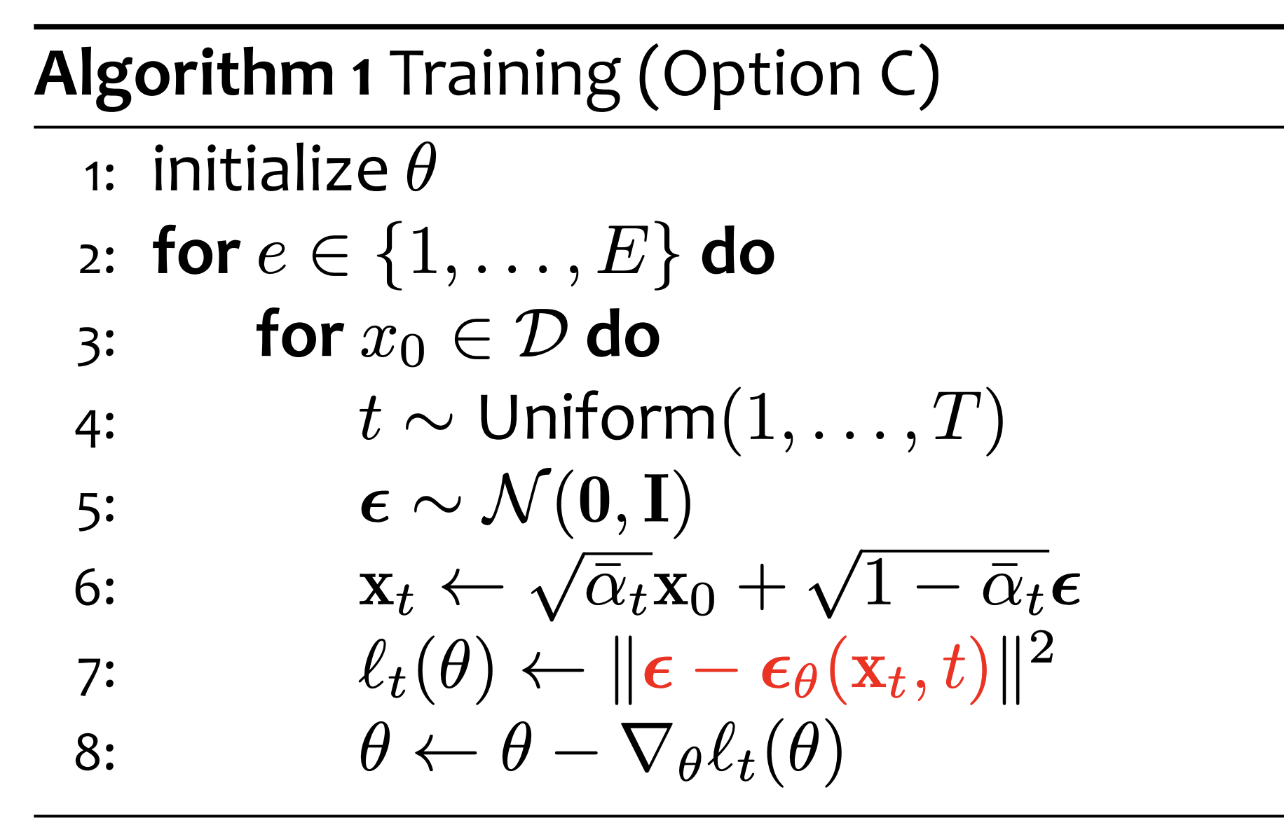
#### Training Algorithm
We present the following algorithm:
[Gormley, 2025, *Lecture 7: Diffusion Models*]
For each of our epochs, we do the following:
1. We sample a timestep $ t $ uniformly
2. We sample some noise $ \epsilon $ from a Unit Gaussian distribution
3. We compute the noised $ x_t $ using our distribution $ q(x_t \mid x_0) $ which we have derived
4. We compute the MSE between our sampled noise and our noise network predictor
5. We do a step with our optimizer (gradient descent) on our model parameters $ \theta $
📝 There are a few things to note here. For one, note how we sample $ x_t $ from the distribution $ q(x_t \mid x_0) \sim \mathcal{N}(\sqrt{\bar{\alpha}_t}x_0, (1 - \bar{\alpha}_t)I) $. We do this with our "reparameterization trick" where we just split the mean and sample unit gaussian noise $ \epsilon $. Why is this a label for $ \epsilon_\theta $? Remember that $ \epsilon_\theta $ is predicting the noise that takes us **all the way back** to $ x_0 $, not just $ x_{t - 1} $.
Notice how we also sample a timestep $ t $ uniformly. This is because we are using just **one** network for *every* single timestep. So we have to ensure that we are learning how to predict the noise from each timestep.
### How Exactly Do Diffusion Models Generate Stuff?
Alright, we have a trained Diffusion model. Now how can we sample from it?
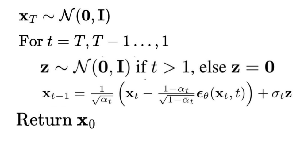
[Cornell University, 2025, *CS 4782: Week 9 Lecture Slides*]
Recall that $ q(x_T) \sim \mathcal{N}(0, 1) $, which was due to our noise schedule and the prior matching term. Now, we can sample unit gaussian noise $ x_T $. ❓But why do we sample $ z \sim \mathcal{N}(0, 1) $? From (12), we saw
$$
q(x_{t - 1} \mid x_t, x_0) \propto \mathcal{N}(x_{t - 1}; \underbrace{\frac{\sqrt{\alpha_t}(1 - \bar{\alpha}_{t - 1})x_{t} + \sqrt{\bar{\alpha}_{t - 1}}(1 - \alpha_t)x_0}{1 - \bar{\alpha}_t}}_{\mu_q(x_t, x_0)}, \underbrace{\frac{(1 - \alpha_t)(1 - \bar{\alpha}_{t - 1})}{1 - \bar{\alpha_t}}}_{\Sigma_q(t)}).
$$
Also, recall from above that $ x_0 = \frac{x_t - \sqrt{1 - \bar{\alpha}_t}\epsilon_0}{\sqrt{\bar{\alpha}_t}} $ (rearranging the closed-form sampling from $ q(x_t \mid x_0) $). So, observe that:
$$
\begin{align}
\mu_q(x_t, x_0) & = \frac{\sqrt{\alpha_t}(1 - \bar{\alpha}_{t - 1})x_{t} + \sqrt{\bar{\alpha}_{t - 1}}(1 - \alpha_t)x_0}{1 - \bar{\alpha}_t} \\
& = \frac{\sqrt{\alpha_t}(1 - \bar{\alpha}_{t - 1})x_{t} + \sqrt{\bar{\alpha}_{t - 1}}(1 - \alpha_t)\frac{x_t - \sqrt{1 - \bar{\alpha}_t}\epsilon_0}{\sqrt{\bar{\alpha}_t}}}{1 - \bar{\alpha}_t} \tag{Plugging in for $ x_0 $} \\
& = \frac{\sqrt{\alpha_t}(1 - \bar{\alpha}_{t - 1})x_{t} + \sqrt{\bar{\alpha}_{t - 1}}(1 - \alpha_t)\frac{x_t - \sqrt{1 - \bar{\alpha}_t}\epsilon_0}{\sqrt{\bar{\alpha}_t}}}{1 - \bar{\alpha}_t} \\
& = \frac{1}{1 - \bar{\alpha}_t}\left(\sqrt{\alpha_t}x_t - \sqrt{\alpha_t}\bar{\alpha}_{t - 1}x_t + \frac{1}{\sqrt{\bar{\alpha}_t}}\left(\sqrt{\bar{\alpha}_{t - 1}}x_t - \sqrt{\bar{\alpha}_{t - 1}}\alpha_tx_t - \sqrt{\bar{\alpha}_{t - 1}}\sqrt{1 - \bar{\alpha}_t}\epsilon_0 + \sqrt{\bar{\alpha}_{t - 1}}\alpha_t\sqrt{1 - \bar{\alpha}_t}\epsilon_0\right)\right) \\
& = \frac{1}{1 - \bar{\alpha}_t}\left(\frac{1}{\sqrt{\alpha_t}}\left(\alpha_tx_t - \alpha_t\bar{\alpha}_{t - 1}x_t + x_t - \alpha_tx_t - \sqrt{1 - \bar{\alpha}_t}\epsilon_0 + \alpha_t\sqrt{1 - \bar{\alpha}_t}\epsilon_0\right)\right) \\
& = \frac{1}{1 - \bar{\alpha}_t}\left(\frac{1}{\sqrt{\alpha_t}}\left(\alpha_tx_t - \bar{\alpha}_{t}x_t + x_t - \alpha_tx_t - \sqrt{1 - \bar{\alpha}_t}\epsilon_0 + \alpha_t\sqrt{1 - \bar{\alpha}_t}\epsilon_0\right)\right) \\
& = \frac{1}{1 - \bar{\alpha}_t}\left(\frac{1}{\sqrt{\alpha_t}}\left(\left(\alpha_t - \bar{\alpha}_{t} + 1 - \alpha_t\right)x_t - \left(\sqrt{1 - \bar{\alpha}_t} - \alpha_t\sqrt{1 - \bar{\alpha}_t}\right)\epsilon_0\right)\right) \\
& = \frac{1}{1 - \bar{\alpha}_t}\left(\frac{1}{\sqrt{\alpha_t}}\left(\left(1 - \bar{\alpha}_t\right)x_t - \left(1 - \alpha_t\right)\sqrt{1 - \bar{\alpha}_t}\epsilon_0\right)\right) \\
& = \frac{1}{\sqrt{\alpha}_t}\left(x_t - \frac{(1 - \alpha_t)}{\sqrt{1 - \bar{\alpha}_t}}\epsilon_0\right)
\end{align}
$$
Hence,
1. Using the above derivation, we plug in $ \epsilon_\theta(x_t, t) $ as our noise estimate for $ \epsilon_0 $.
2. We obtain $ \mu_q(x_t, x_0) $ as a result (a prediction for the real mean of $ q(x_{t - 1} \mid x_t, x_0) $.
3. We note that $ \sigma_t = \Sigma_q(t) = \frac{(1 - \alpha_t)(1 - \bar{\alpha}_{t - 1})}{1 - \bar{\alpha_t}} $ from before (from our deterministic noise schedule), and this is independent of $ x_0 $.
4. Now that we have the mean, we use our "reparameterization trick" to sample from $ q(x_{t - 1} \mid x_t, x_0) $, i.e. $ x_{t - 1} = \underbrace{\frac{1}{\sqrt{\alpha}_t}\left(x_t - \frac{(1 - \alpha_t)}{\sqrt{1 - \bar{\alpha}_t}}\epsilon_0\right)}_{\mu_q(x_t, x_0)} + \underbrace{\frac{(1 - \alpha_t)(1 - \bar{\alpha}_{t - 1})}{1 - \bar{\alpha_t}}}_{\sigma_t}z $.
5. We repeat this until we sample our $ x_1 $.
Once we have $ x_1 $, we just take the estimated mean $ \mu_q $ as our estimate for $ x_0 $ and **do not add any more noise** for sampling because we just want a clean image as our output!
💡 **Key Insight:** If we had trained our network to predict $ \mu_\theta(x_t, x_0) $, we would not have needed all this extra math above and could just use $ \sigma_t $ directly! But we resort to $ \epsilon_\theta(x_t, t) $ for the empirical boost in performance.
### Applications of Diffusion Models
Diffusion models are powerful generative tools used across a variety of domains:
- 🖼 **Image Generation**: Models like *DALL·E*, *Imagen*, and *Stable Diffusion* generate high-quality, photorealistic images.
- 🎨 **Image Editing**: Used for inpainting, outpainting, and style transfer by completing or modifying images.
- 🗣 **Text-to-Image**: Cross-modal models condition on text prompts to generate semantically aligned visuals.
- 🎵 **Audio Synthesis**: Applied to speech and music generation (e.g. *DiffWave*).
- 🧬 **Scientific Design**: Enable structure generation for proteins, molecules, and materials.
- 🧠 **Medical Imaging**: Improve or synthesize diagnostic images for augmentation and analysis.
> **Why so popular?** They combine stability, diversity, and quality, and work well with conditioning and pretrained embeddings.
#### Downsides?
There are a couple downsides to DDPMs:
1. The major downside of DDPMs is that they are very *computationally expensive*. In particular, $ T $ is usually on the order of thousands, so learning the reverse model is nontrivial! To just sample **one** image, we have to do **thousands** of denoising steps. (❕ We will see a remedy to this with Cold Diffusion and DDIMs in *Diffusion II*, or you can read about them in [12]).
2. Raw DDPMs are also random and while effective, can generate images that do not align with the intention. (❕ We will learn more about how to control generation with conditioning in *Diffusion II*).
## References
[1] Lugmayr, A., Danelljan, M., Romero, A., & Timofte, R. (2022). *RePaint: Inpainting using denoising diffusion probabilistic models*. arXiv preprint arXiv:2208.11970. [PDF](https://arxiv.org/pdf/2208.11970)
[2] Ho, J., Jain, A., & Abbeel, P. (2020). Denoising diffusion probabilistic models. *Advances in Neural Information Processing Systems, 33*, 6840–6851. [arXiv](https://arxiv.org/abs/2006.11239)
[3] Saharia, C., Chan, W., Saxena, S., Li, L., Whang, J., Denton, E., Seyed Ghasemipour, S. K., Karagol Ayan, B., Mahdavi, S. S., Gontijo Lopes, R., et al. (2022). *Photorealistic text-to-image diffusion models with deep language understanding*. arXiv preprint arXiv:2205.11487. [arXiv](https://arxiv.org/abs/2205.11487)
[4] CVPR 2022 Tutorial. *Diffusion Models*. [Website](https://cvpr2022-tutorial-diffusion-models.github.io/)
[5] Blei, D. M. (2021). Variational inference: Foundations and methods. In *Probabilistic Machine Learning: Advanced Topics* (pp. 89–116). Springer. [Link](https://link.springer.com/chapter/10.1007/978-3-030-93158-2_4)
[6] Gormley, M., Virtue, P. (2025). Lecture 7: Diffusion Models. *Carnegie Mellon University, 10-423 Course Slides*. [PDF](https://www.cs.cmu.edu/~mgormley/courses/10423//slides/lecture7-diffusion.pdf)
[7] Stanford University. (2023). *CS231n: Convolutional Neural Networks for Visual Recognition – Lecture 15*. [PDF](https://cs231n.stanford.edu/slides/2023/lecture_15.pdf)
[8] Esteve, J. (2018). About generative and discriminative models. *Medium*. [Article](https://medium.com/@jordi299/about-generative-and-discriminative-models-d8958b67ad32)
[9] Cornell University. (2020). Training and GANs – Part 2. *CS5670 Course Materials*. [PDF](https://www.cs.cornell.edu/courses/cs5670/2020sp/lectures/TrainingAndGANS_part2_web.pdf)
[10] Erdem, K. (2022). Step-by-step visual introduction to diffusion models. *Medium*. [Article](https://medium.com/@kemalpiro/step-by-step-visual-introduction-to-diffusion-models-235942d2f15c)
[11] Cornell University. (2025). *CS 4782: Week 9 Lecture Slides*. [PDF](https://www.cs.cornell.edu/courses/cs4782/2025sp/slides/pdf/week9_1_slides.pdf)
[12] Ramesh, A., Dhariwal, P., Nichol, A., Chu, C., & Chen, M. (2022). *Hierarchical text-conditional image generation with clip latents*. arXiv preprint arXiv:2208.09392. [arXiv](https://arxiv.org/abs/2208.09392)
[13] Gainetdinov, A. (2024). *Understanding GAN Mode Collapse: Causes and Solutions*. [Article](https://hackernoon.com/understanding-gan-mode-collapse-causes-and-solutions)
[14] Weng, L. (2021). *Diffusion Models: A Comprehensive Survey*. [Website](https://lilianweng.github.io/posts/2021-07-11-diffusion-models/)
$$
$$