# Reinforcement Learning: MDPs, Value, and Policy
## 1 Comparison: Supervised, Unsupervised, and Reinforcement Learning
Machine learning paradigms differ in the type of feedback available and their learning objective.
| Paradigm | Data / Feedback | Goal | Typical Tasks | Example |
| ----------------- | --------------------------------- | ---------------------------------------------- | ----------------------------- | -------------------- |
| **Supervised** | Labeled data (input–output pairs) | Learn a mapping from inputs to outputs | Classification, regression | Spam detection |
| **Unsupervised** | Unlabeled data (inputs only) | Discover hidden structure or patterns | Clustering, generative models | Image compression |
| **Reinforcement** | Delayed scalar reward signals | Learn a policy to maximize cumulative reward | Game-playing, robotics | Autonomous driving |
### 1.1 Why Not Just Use Supervised Learning?
Consider tasks like flying a helicopter upside-down or having a robot learn to pick up blocks. In these settings:
- There is **no dataset of "correct" actions** to learn from.
- Feedback is **delayed** — a reward may come only after a long sequence of actions (e.g., winning or losing a chess game). This is the **Reward Assignment Problem**: which of the many actions caused the agent to win or lose?
- The agent's actions **change the environment**, so future data depends on current decisions.
Reinforcement Learning (RL) fills this gap by letting an **agent** learn through trial-and-error interaction with an **environment**.
---
## 2 Reinforcement Learning (Core Concepts)
> *"The reinforcement learning problem is meant to be a straightforward framing of the problem of learning from interaction to achieve a goal."*
> — Sutton & Barto, *Reinforcement Learning: An Introduction*
### 2.1 The Agent–Environment Loop
At each time step $ t $:
1. The agent observes the current **state** $ S_t $.
2. The agent selects an **action** $ A_t $ according to its **policy**.
3. The environment returns a **reward** $ R_{t+1} $ and transitions to a new **state** $ S_{t+1} $.
This loop repeats, possibly ending when a **terminal state** is reached.
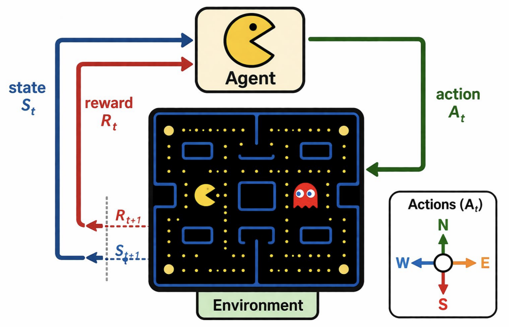
**Key components:**
- **Agent:** Perceives the environment, makes decisions, and aims to maximize reward.
- **Environment:** The external context the agent operates in; provides state information and reward feedback.
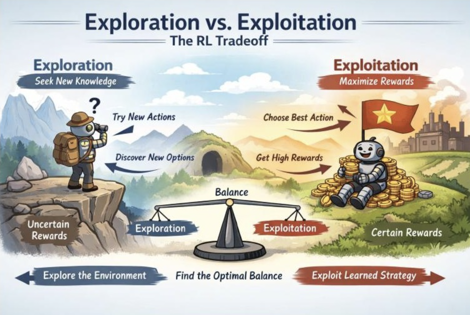
### 2.2 Exploration vs. Exploitation
Unlike supervised learning, an RL agent has no teacher providing correct actions. It must balance two competing goals:
- **Exploration:** Trying new, potentially suboptimal actions to discover better strategies.
- **Exploitation:** Using current knowledge to take the best-known action and accumulate reward.
A common approach is **ε-greedy** exploration:
- With probability **ε**, take a random action (explore).
- Otherwise, take the action with the highest estimated value: $ \arg\max_a Q(s, a) $ (exploit).
Typically ε is slowly decreased over time so the agent explores broadly early on and converges to a refined policy later.
---
## 3 Markov Decision Processes (MDPs)
A **Markov Decision Process** is the standard mathematical framework for formalizing RL environments. An MDP models sequential decision-making where outcomes are **partly random** and **partly under the control** of a decision-maker.
An MDP is defined by the tuple (S, A, P, R, γ):
### 3.1 State Space (S)
$$\mathcal{S} = \{s_1, s_2, s_3, \dots\}$$
The set of all possible states representing the environment. A state $ s \in \mathcal{S} $ captures **everything the agent needs to know** about the current situation — position of the agent, enemies, walls, etc. States can be discrete or continuous.
### 3.2 Action Space (A)
$$\mathcal{A} = \{\text{Up, Down, Left, Right}\}$$
The set of all actions the agent can take. In more complex environments, actions may be continuous (e.g., torque applied to a robot joint).
### 3.3 Transition Function (P)
The transition probability function $ \mathcal{P}(s' \mid s, a) $ gives the probability of moving to state $ s' $ when the agent takes action $ a $ in state $ s $.
> **The Markov Property:** The next state depends *only* on the current state and action, not on any prior history:
>
> $$P(S_{t+1} = s' \mid S_t = s, A_t = a, S_{t-1}, A_{t-1}, \dots, S_0) = P(S_{t+1} = s' \mid S_t = s, A_t = a)$$
>
> This memoryless property means all relevant information from the history is encapsulated in the current state.
### 3.4 Reward Function (R)
$$\mathcal{R}(s, a, s')$$
The immediate numerical reward received when the agent transitions from state $ s $ to state $ s' $ via action $ a $. Rewards can be positive (reinforcing) or negative (punishing).
**Examples:** +1 for collecting a gold coin, +100 for finishing a game, −100 for dying. Most settings include a small negative reward per step (e.g., −0.03) to encourage the agent to finish quickly.
**Dense vs. Sparse Rewards:**
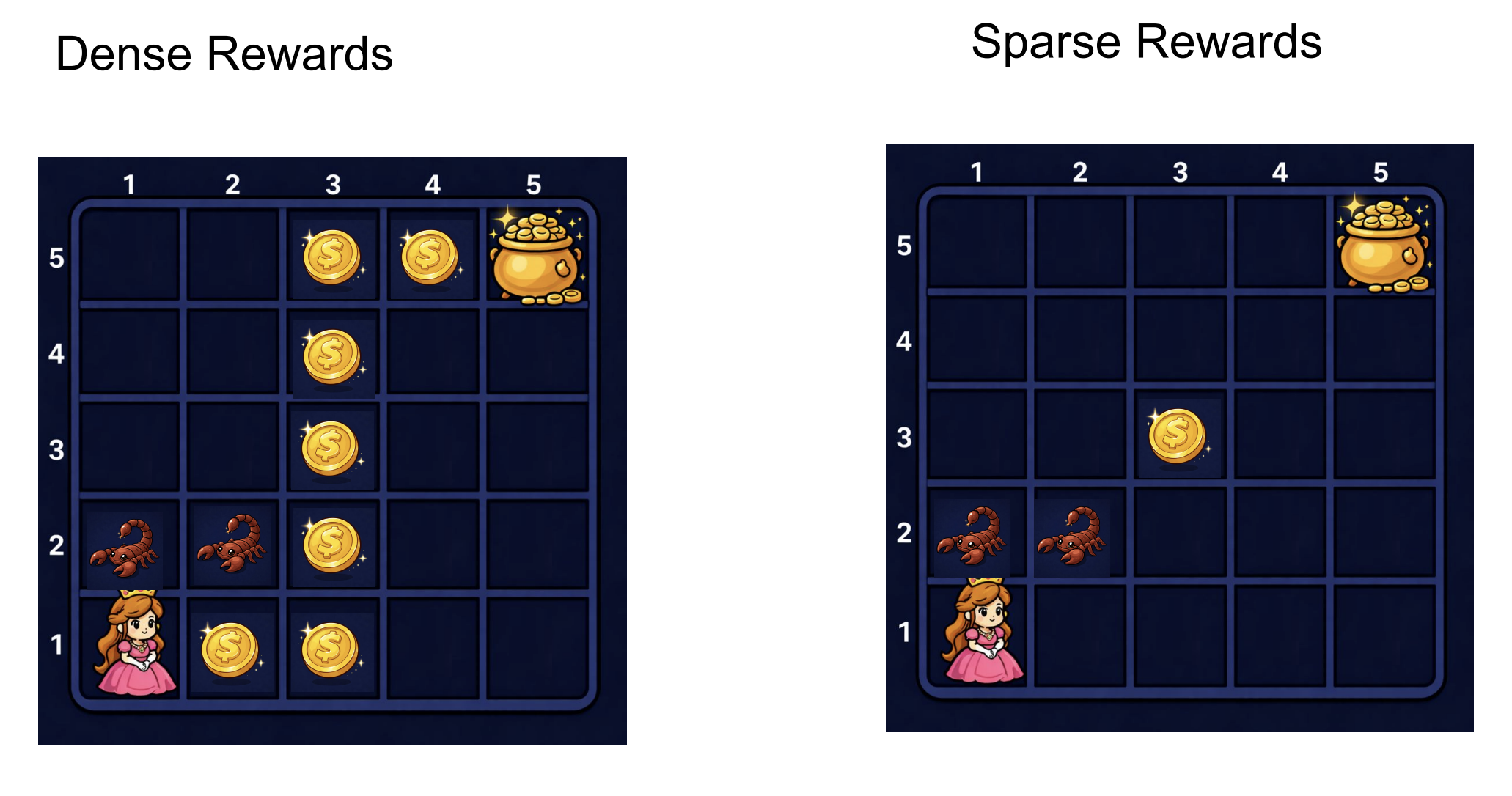
*Left: Dense rewards — many coins scattered along the path provide frequent feedback. Right: Sparse rewards — only a couple of reward signals exist, making learning significantly harder.*
### 3.5 Discount Factor (γ)
$$\gamma \in [0, 1]$$
The discount factor determines how much the agent values future rewards relative to immediate ones. The **return** $ G_t $ (total discounted reward from time $ t $ onward) is:
$$G_t = \sum_{k=0}^{\infty} \gamma^k R_{t+k+1}$$
**Intuition for different values of $ \gamma $:**
| $ \gamma $ value | Behavior |
|---|---|
| Close to **1** (e.g., 0.99) | Far-sighted — cares almost equally about immediate and distant rewards |
| Close to **0** | Myopic — focuses almost entirely on immediate reward |
| Exactly **1** | All future rewards weighted equally (can diverge in non-episodic tasks) |
| Exactly **0** | Only considers the very next reward |
> **Example:** With γ = 0.95, a reward of 1 received 10 steps in the future has a present value of about 0.60. The agent gives **nearly equal weight** to immediate and future rewards, slightly preferring sooner ones.
### 3.6 Grid-World Example

**MDP specification for this grid:**
- **State** = grid cell coordinate, e.g., (row, col).
- **Actions** = {Up, Down, Left, Right}.
- **Transition** = 80% intended direction, 10% each perpendicular direction (slippery floor). Hitting a wall keeps the agent in place.
- **Reward** = +1 (Mario), −1 (Bowser), −0.03 per step elsewhere.
- **$ \gamma $** ≈ 0.9.
---
## 4 Policy
A **policy** $ \pi $ defines the agent's strategy: how it chooses actions in each state. Formally, $ \pi(a \mid s) $ gives the probability of selecting action $ a $ in state $ s $.
We want an **optimal policy** $ \pi^*: S \to A $ that maximizes expected cumulative reward from every state.
### 4.1 Deterministic Policies
A deterministic policy maps each state to a single action: $ a = \pi(s) $. For example, "in cell (3, 2), always move Right."
For any finite MDP there always exists an optimal policy that is deterministic and stationary (depends only on the current state, not on time or history). This is a consequence of the Markov property and the principle of optimality.
### 4.2 Stochastic Policies
A stochastic policy assigns a probability distribution over actions for each state. For example, in state $ s $ the policy might assign probability $ 0.7 $ to moving Right and probability $ 0.3 $ to moving Up. These are useful for exploration and are sometimes necessary in competitive or partially observable settings.
Stochastic policies generalize deterministic ones: a deterministic policy is simply a stochastic policy concentrated on a single action. In practice, policies are often initialized as stochastic and gradually become more deterministic as the agent learns.
### 4.3 Optimal Policy Example

Different reward structures produce different optimal policies. With step cost −0.03, the policy directs the agent along the top row toward +1, avoiding cells adjacent to Bowser. With a much larger step cost, the agent may rush toward the nearest terminal — even Bowser — just to stop accumulating penalties.
---
## 5 Value Functions
Value functions assign a number to each state (or state–action pair) representing how good it is for the agent to be there. **Optimal values define optimal policies.**
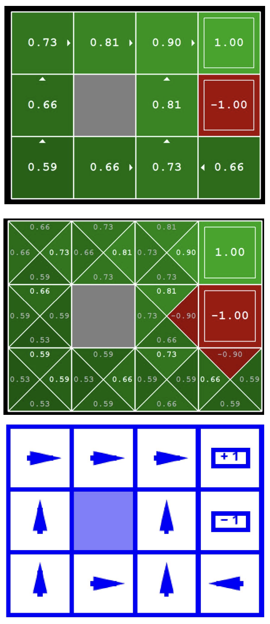
*From top to bottom: the optimal state-value function V\* (one value per cell), the optimal action-value function Q\* (four Q-values per cell, one per action), and the resulting optimal policy π\* (arrows showing the best action).*
### 5.1 State-Value Function ($ V $)
The **state-value function** for policy $ \pi $, denoted $ V^\pi(s) $, is the expected return when starting in state $ s $ and following $ \pi $ thereafter:
$$V^\pi(s) = \mathbb{E}_\pi\!\left[\sum_{k=0}^{\infty} \gamma^k R_{t+k+1} \;\middle|\; S_t = s\right]$$
$ V^\pi(s) $ measures "how good is it to be in state $ s $ under policy $ \pi $."
**Two important cases:**
- **Fixed (sub-optimal) policy** $ V^\pi(s) $: Expected reward starting in $ s $ and always following $ \pi $ (even if $ \pi $ is not the best).
- **Optimal value** $ V^*(s) = \max_\pi V^\pi(s) $: Expected reward starting in $ s $ and acting optimally.
### 5.2 Bellman Expectation Equation (for a fixed policy)
The value function satisfies a recursive relationship. At time $ t $, $ G_t = R_{t+1} + \gamma G_{t+1} $, so:
$$V^\pi(s) = \mathbb{E}\!\left[R_{t+1} + \gamma\, V^\pi(S_{t+1}) \;\middle|\; S_t = s\right]$$
Expanding over all actions and next states:
$$V^\pi(s) = \sum_{a \in \mathcal{A}} \pi(a \mid s) \sum_{s' \in \mathcal{S}} \mathcal{P}(s' \mid s, a)\left[\mathcal{R}(s, a, s') + \gamma\, V^\pi(s')\right]$$
This says: the value of a state equals the expected immediate reward plus the discounted value of the next state, averaged over the agent's action choices and the environment's transitions.
---
## 6 Action-Value Function (Q-Function)
The **action-value function** (or **Q-function**) for policy $ \pi $ is:
$$Q^\pi(s, a) = \mathbb{E}\!\left[G_t \;\middle|\; S_t = s,\, A_t = a,\; \text{follow } \pi \text{ after}\right]$$
$ Q^\pi(s, a) $ measures "how good is it to take action $ a $ in state $ s $ and then follow $ \pi $." The "Q" stands for *quality*.
The relationship between $ V $ and $ Q $:
$$V^\pi(s) = \sum_{a \in \mathcal{A}} \pi(a \mid s)\, Q^\pi(s, a)$$
For a deterministic policy: $ V^\pi(s) = Q^\pi(s, \pi(s)) $.
**Optimal Q-function:**
$$Q^*(s, a) = \max_\pi Q^\pi(s, a)$$
Once you have $ Q^* $, recovering the optimal policy is trivial:
$$\pi^*(s) = \arg\max_a Q^*(s, a)$$
This is why Q-values are so central to RL — **actions are easier to select from Q-values than from V-values**, which additionally require knowledge of the transition model to do a one-step lookahead.
---
## 7 Bellman Optimality Equations
The Bellman optimality equations give the recursive relationship that the optimal value functions must satisfy.
### 7.1 Derivation
**Step 1 — Definitions:**
$$V^*(s) = \max_\pi \mathbb{E}_\pi[G_t \mid S_t = s] \qquad Q^*(s,a) = \max_\pi \mathbb{E}_\pi[G_t \mid S_t = s, A_t = a]$$
**Step 2 — Linking $ V^* $ and $ Q^* $:** The best thing to do in state $ s $ is pick the action with the highest $ Q^* $:
$$V^*(s) = \max_a\; Q^*(s, a)$$
**Step 3 — Expanding $ Q^* $:** Using $ G_t = R_{t+1} + \gamma G_{t+1} $ and the Markov property:
$$Q^*(s, a) = \sum_{s'} \mathcal{P}(s' \mid s, a)\left[\mathcal{R}(s, a, s') + \gamma\, V^*(s')\right]$$
**Step 4 — Substituting** step 2 into step 3:
$$\boxed{V^*(s) = \max_a \sum_{s'} \mathcal{P}(s' \mid s, a)\left[\mathcal{R}(s, a, s') + \gamma\, V^*(s')\right]}$$
This is the **Bellman optimality equation for $ V^* $**: the optimal value of a state equals the best action's expected immediate reward plus the discounted optimal value of the resulting next state.
---
## 8 Value Iteration
Value iteration computes $ V^* $ (and thus $ \pi^* $) by repeatedly applying the Bellman update.
**Algorithm:**
1. Initialize $ V_0(s) = 0 $ for all states $ s $.
2. For each iteration $ i $, update every state:
$$
V_{i+1}(s) \leftarrow \max_a \sum_{s'} \mathcal{P}(s' \mid s, a)\left[\mathcal{R}(s, a, s') + \gamma\, V_i(s')\right]
$$
3. Repeat until convergence: $ |V_{i+1}(s) - V_i(s)| < \epsilon $ for all $ s $.
**Theorem:** Value iteration converges to the unique optimal values $ V^* $. The policy often converges long before the values do.
### 8.1 Worked Example

Consider state $ \langle 3, 3 \rangle $ (one step left of the +1 goal). The max is achieved by action = Right:
$$V_2(\langle 3,3 \rangle) = 0.8 \times \left[0 + 0.9 \times 1\right] + 0.1 \times \left[0 + 0.9 \times 0\right] + 0.1 \times \left[0 + 0.9 \times 0\right] = 0.72$$
After ~100 iterations, the values converge fully:

### 8.2 Computing the Policy from Values
**From $ V^* $** (requires knowing the transition model):
$$\pi^*(s) = \arg\max_a \sum_{s'} \mathcal{P}(s' \mid s, a)\left[\mathcal{R}(s, a, s') + \gamma\, V^*(s')\right]$$
**From $ Q^* $** (no model needed — just pick the max):
$$\pi^*(s) = \arg\max_a\; Q^*(s, a)$$
**Lesson:** Actions are easier to select from Q-values!
---
## 9 Policy Iteration
An alternative to value iteration is **policy iteration**, which alternates two steps:
**Step 1 — Policy Evaluation:** Given a fixed policy $ \pi_k $, compute $ V^{\pi_k} $ by iterating the simplified (no max) Bellman update until convergence:
$$V_{i+1}^{\pi_k}(s) \leftarrow \sum_{s'} T(s, \pi_k(s), s')\left[R(s, \pi_k(s), s') + \gamma\, V_i^{\pi_k}(s')\right]$$
**Step 2 — Policy Improvement:** Use the converged values to find a better policy via one-step lookahead:
$$\pi_{k+1}(s) = \arg\max_a \sum_{s'} T(s, a, s')\left[R(s, a, s') + \gamma\, V^{\pi_k}(s')\right]$$
Repeat steps 1 and 2 until the policy no longer changes. Policy iteration is guaranteed to converge to $ \pi^* $.
---
## 10 Scalability Challenges
### 10.1 State-Space Explosion
Real environments have enormous state spaces. For Pac-Man with 100 board positions, 4 ghosts, and Pac-Man: $ |S| = 100^5 = 10^{10} $. Including 100 pellets (each eaten or not): $ 2^{100} \times 10^{10} > 10^{40} $ states. Tabular methods become completely infeasible.
> **Practice problem:** A 10×10 grid with 5 fixed obstacles, 1 fixed goal, and 4 agent orientations has $ 100 \times 4 = 400 $ states. Since obstacles and goal positions are fixed, the state is fully determined by the agent's cell and orientation.
### 10.2 Sparse Rewards
When only terminal states give ±1 and all other rewards are zero, the agent receives almost no learning signal during exploration. **Reward shaping** (adding small intermediate rewards) helps address this.
### 10.3 Unknown Dynamics
In most real-world problems, $ \mathcal{P} $ and $ \mathcal{R} $ are unknown. The agent must learn from experience, leading to **model-free** methods like Q-learning and policy gradient algorithms.
### 10.4 Looking Ahead: Deep RL

To handle large state spaces, we replace the Q-table with a neural network that approximates $ Q(s, a) $ — this is **Deep Q-Learning (DQN)**. Instead of storing a value for every state–action pair, the network takes the state as input and outputs Q-values for all actions, enabling generalization across similar states.
---
## 11 Summary
- **Reinforcement Learning** is learning from delayed reward signals through trial-and-error interaction.
- **MDPs** formalize RL with the tuple $ \langle \mathcal{S}, \mathcal{A}, \mathcal{P}, \mathcal{R}, \gamma \rangle $. The Markov property ensures the next state depends only on the current state and action.
- A **policy** $ \pi $ maps states to actions. The **optimal policy** $ \pi^* $ maximizes expected cumulative reward.
- The **value function** $ V^\pi(s) $ measures expected return from state $ s $ under $ \pi $. The **Q-function** $ Q^\pi(s,a) $ measures expected return from taking action $ a $ in state $ s $ then following $ \pi $.
- **Bellman equations** express optimal values recursively.
- **Value iteration** and **policy iteration** compute optimal values and policies.
- Practical RL must handle large state spaces, sparse rewards, and unknown dynamics — motivating **deep RL** and smart **exploration**.
---
## References
- Sutton & Barto, *Reinforcement Learning: An Introduction* (2nd ed.) — [PDF](https://web.stanford.edu/class/psych209/Readings/SuttonBartoIPRLBook2ndEd.pdf)
- CS 4782 Deep Learning, Cornell — Week 8 Lecture Slides (MDPs / Value)