# Deep Q-Learning
## 1 Value Iteration (Model-Based)
Recall that we are trying to find an optimal policy $ \pi^*(s) $ that decides the best action to take in a given state. Last lecture, we used a value function $ V(s) $ to simulate that policy.
$$V^*(s)=\text{expected reward starting in } s \text{ while acting optimally}$$
Value iteration repeatedly updates these values by applying the Bellman update:
$$V_{i+1}(s) \leftarrow \max_{a} \sum_{s'} \mathcal{P}(s' \mid s, a) \left[ \mathcal{R}(s, a, s') + \gamma V_i(s') \right]$$
The nice thing about value iteration is it's guaranteed to converge to the unique optimal values $ V^* $. Seems great, but there are some problems with the approach.
1. First, value iteration requires us to know the probability of every transition $ \mathcal{P}(s' \mid s, a) $ and the reward for every transition $ \mathcal{R}(s, a, s') $. In most real problems, these dynamics are **unknown** or too complex to capture. It's hard to write down the exact physics of a robot's environment or to know how a financial market will behave.
2. Second, value iteration is quite expensive. At every iteration, we update all states for all actions which works out to $ O(|S||A|) $ per iteration. For continuous state/action spaces, it's infeasible to update, much less store the value table. Even in discrete state space problems like Pac-Man, there are $ 2^{240} $ states from dot configurations alone.
With all these problems, how can we proceed? Let's tackle the first problem, well first. Model-based approaches like value iteration require us to model the environment which turns out to be hard if not impossible. But thinking back to our original goal; we only wanted to find the optimal policy, we never cared about modeling the environment. So what if we didn't? Enter Q-Learning, a model-free approach.
## 2 Q-Learning (Model-Free)
Recall the definition of a Q-value.
$$Q(s,a) = \text{expected reward starting in state } s \text{ and taking action } a$$
The motivation behind Q-Learning is similar to stochastic gradient descent, where we make updates based on a single noisy sample rather than finding the true gradient over all data. We learn from experience to avoid an expensive computation over all states:
>1: Initialize $ Q(s, a) $ for all $ s, a $; set $ Q(\text{terminal}, \cdot) = 0 $
2: Repeat (for each episode):
3: Initialize state $ s $
4: Repeat (for each step):
5: Choose action $ a $ from $ s $ using $ \epsilon $-greedy policy
6: Take action $ a $, observe reward $ R $ and next state $ s' $
7: Update the value function:
$$Q(s, a) \leftarrow (1 - \alpha)Q(s, a) + \alpha \left[ R + \gamma \max_{a'} Q(s', a') \right]$$
8: $ s \leftarrow s' $
9: Until $ s $ is terminal
It might seem a little complicated but it boils down to acting in the environment, observing what happened, and using that to update our Q-value.
#### 2.1 Q-Value Update
Let's break down the Q-value update expression $ Q(s, a) \leftarrow (1 - \alpha)Q(s, a) + \alpha \left[ R + \gamma \max_{a'} Q(s', a') \right] $
* $ (1−\alpha)Q(s,a) $ is reminiscent of Adam where we "remember" most of the old estimate
* $ \alpha $ is our learning rate, the higher it is the more we update
* $ R(s_t,a_t,s_t')+\gamma \underset{a'}\max Q(s',a') $ is our guess of the true Q-value: the reward we get plus the discounted value of the best thing we can do from $ s' $.
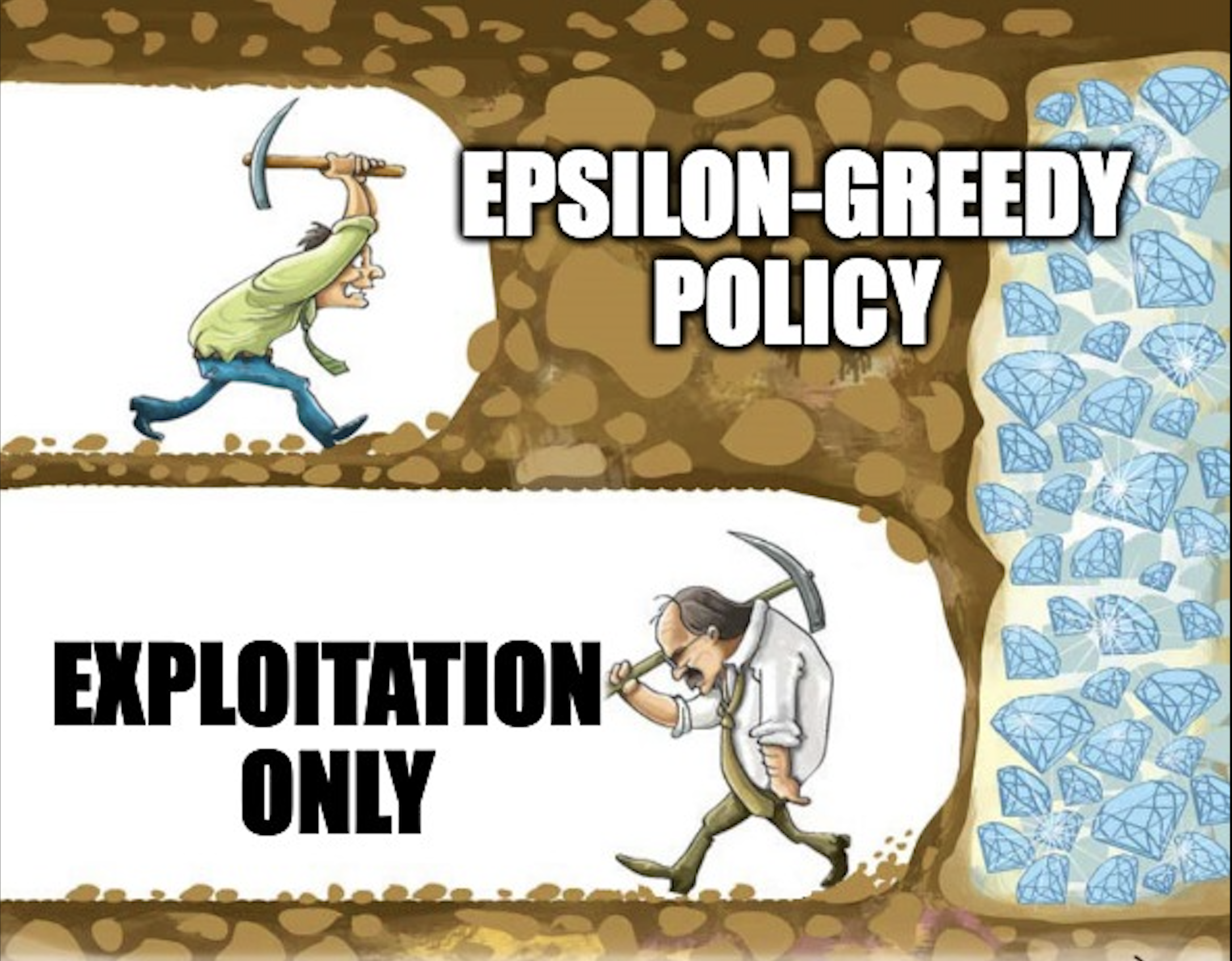
#### 2.2 $ \epsilon $-greedy Policy
Next question: how do we choose actions? We need to balance between using our known Q-values to take the best action (exploitation) and trying new things to find potentially better actions (exploration). If we always exploit, we might get stuck in a local but not global optimum. If we always explore, we never learn and improve. So some mix of exploitation and exploration is optimal and we commonly handle this tradeoff with an $ \epsilon $-greedy policy:
$$\pi(s)=\begin{cases}\underset{a}\arg\max Q(s,a)\qquad \text{with probability } 1-\epsilon\\\text{random action}\qquad \text{with probability } \epsilon \end{cases}$$
In practice, we decrease $ \epsilon $ over time so we explore a lot at the beginning when we know nothing then exploit more as our Q-value estimates get better.
## 3 From Q-Learning to Deep Q-Learning
Q-Learning solves one problem: we no longer need to iterate over all states and actions in our update loop. But the other half of the problem remains: how do we store the Q-values? For problems with large or continuous state spaces, it's not feasible to fit our Q-values in memory. So what if we just don't? Enter neural networks. By using the insight that similar states should have similar Q-values, we can start to generalize and use neural networks as a function to get a Q-value. There are two approaches on how to set up such a neural network.
1. **state + action as input, one Q-value output**. You feed in the (state, action) pair and get out a singular Q-value. However, this is problematic because you have to run the network $ |A| $ times (once per action) to find the best action.
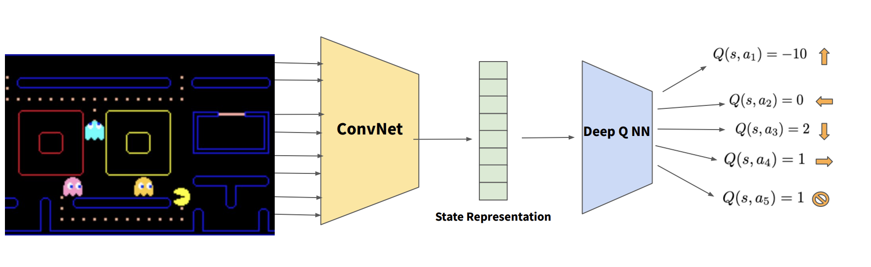
2. **all states as input, all Q-values output**. You feed in the state and get back Q-values for all actions simultaneously. Thus, we only need a singular forward pass to find the best action. This is the preferred approach!! But wait a minute, isn't it easier to parallelize option 1? True, but option 2 is still better as explained here.^[It is true that for option 1, we can parallelize all $ |A| $ passes at the same time, making the time taken similar. However, we still prefer option 2 for a couple reasons. Option 2 networks often look like some convolutional layers to process the state and then a linear layer at the end to output the Q-values. Option 1 networks also need to do the state processing, so when we run the forward pass $ |A| $ times we are redundantly doing the state processing. There are also issues with unclear gradient signal as gradients from different actions are spread across different forward passes. Furthermore, we need to continuously move the large state tensor in and out of the cache which is expensive.]
If we are going with option 2, how do we get the representation of all states? Going back to Pac-Man, we have an image of the game as input but we want the state tensor. We can either 1) carefully design a feature map or just 2) slap some convolutional layers at the front of the network that learn how to output the state tensor.
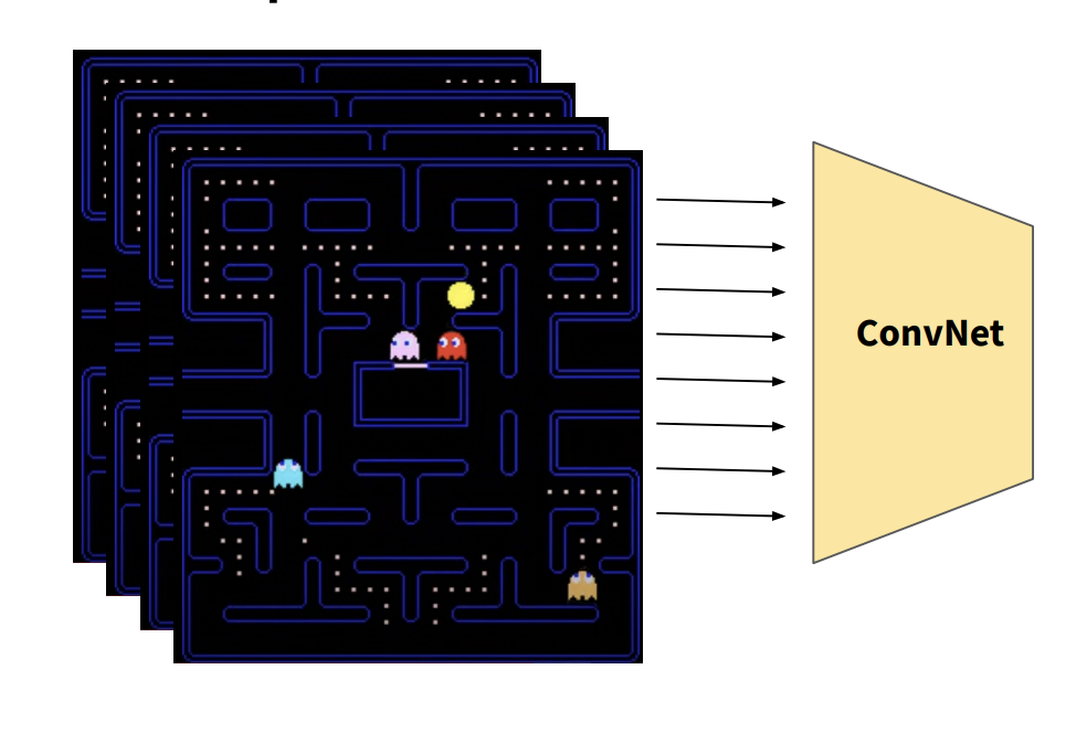
Another problem is that it's hard to infer from a single frame which direction things are moving. Thus, to give a temporal context, Deep Q Networks (DQN) typically stack together the last 4 frames as input to the ConvNet. That way the network can figure out some notion of direction and velocity.
## 4 Training the DQN
#### 4.1 Naive Approach
Now that we've picked our network architecture, how do we actually train it? Naively, we could have the agent take an action, get the observation $ (s,a,r,s') $, do a gradient step, and then repeat in an online SGD fashion.
What's the problem with that naive approach? The samples that we take are highly correlated with each other. $ (s_t, a_t, r_t, s_t') $ and $ (s_{t+1}, a_{t+1}, r_{t+1}, s_{t+1}') $ are nearly identical to each other as the game state barely changed between the two samples. Why is this problematic? When we did analysis on SGD and got guarantees about fast convergence, we assumed that the data was iid (independent and identically distributed). With highly correlated samples, the loss landscape becomes messy and hard to optimize. The signal from gradients point in biased directions rather than averaging to the true data distribution. Convergence may not be guaranteed and the model may struggle to generalize.
#### 4.2 Experience Replay
So, what's the fix? Instead of immediately using the transitions we sample, we store them into a **replay buffer**. So the workflow may look like:
1. Sample many transitions $ (s_t,a_t,r_t,s_t') $ in a replay buffer
2. Sample a random minibatch to train on
3. Perform gradient descent
Minibatches contain transitions from many points in time, reducing the high correlation issue. In addition, by sampling across the whole history of a trajectory, we don't forget earlier experiences. Finally, we can use the same observation multiple times throughout training, improving efficiency.
#### 4.3 Target Network
The issue: **Moving target**
Recall the Q-learning update:
$$Q(s,a) \leftarrow (1-\alpha) Q(s,a) + \alpha \left[R(s,a) + \gamma \underset{a'}\max Q(s',a')\right]$$
Equivalently,
$$Q(s,a) \leftarrow Q(s,a) + \alpha \left[R(s,a) + \gamma \underset{a'}\max Q(s',a') - Q(s,a)\right]$$
At convergence, $ Q(s,a) = R(s,a) + \gamma \underset{a'}\max Q(s',a') $.
Therefore, $ R(s,a) + \gamma \underset{a'}\max Q(s',a') $ is the value that we train the Q-network to approximate. We define it as the Q-target, and minimize the following loss in training:
$$\mathcal{L}(\theta) = \big\|\underbrace{R(s,a) + \gamma \underset{a}\max Q(s',a;\theta)}_{\text{Q-target y}} - Q(s,a;\theta) \big\|^2$$
where $ \theta $ is network parameters.
However, since the target and the Q-function share the same parameters $ \theta $, they are strongly correlated, which makes optimization unstable. An intuitive way to understand this is that when Q is updated to better match the current target, the target itself also changes immediately. As a result, the model is effectively optimizing a changing objective.
The solution: **Frozen target network**
We use a frozen Q-network with parameters $ \theta' $ to compute the target
$$y = R(s,a) + \gamma \underset{a}\max Q(s',a;\theta')$$
The loss then becomes
$$\mathcal{L}(\theta) = \big\|\underbrace{R(s,a) + \gamma \underset{a}\max Q(s',a;\theta')}_{\text{Q-target y}} - Q(s,a;\theta) \big\|^2$$
Since $ \theta $ is being updated while $ \theta' $ is kept fixed, we are optimizing Q to match a fixed target.
However, if the Q-network keeps learning from outdated targets, it may not converge properly. So, we periodically update the target network parameters $ \theta' $ to the current Q-network parameters $ \theta $, e.g. every $ T $ steps. Alternatively, we can use a soft update as shown in the slides: $ \theta' \leftarrow \tau \theta + (1-\tau) \theta' $.
#### 4.4 Putting it Together
Putting everything together, the high-level training loop of DQN is:
- Select action using the $ \epsilon $-greedy policy
- Execute action and store transitions to **replay buffer**
- Sample minibatch from **replay buffer**
- Compute target using **target network**
- Update Q-network
- Periodically update **target network**
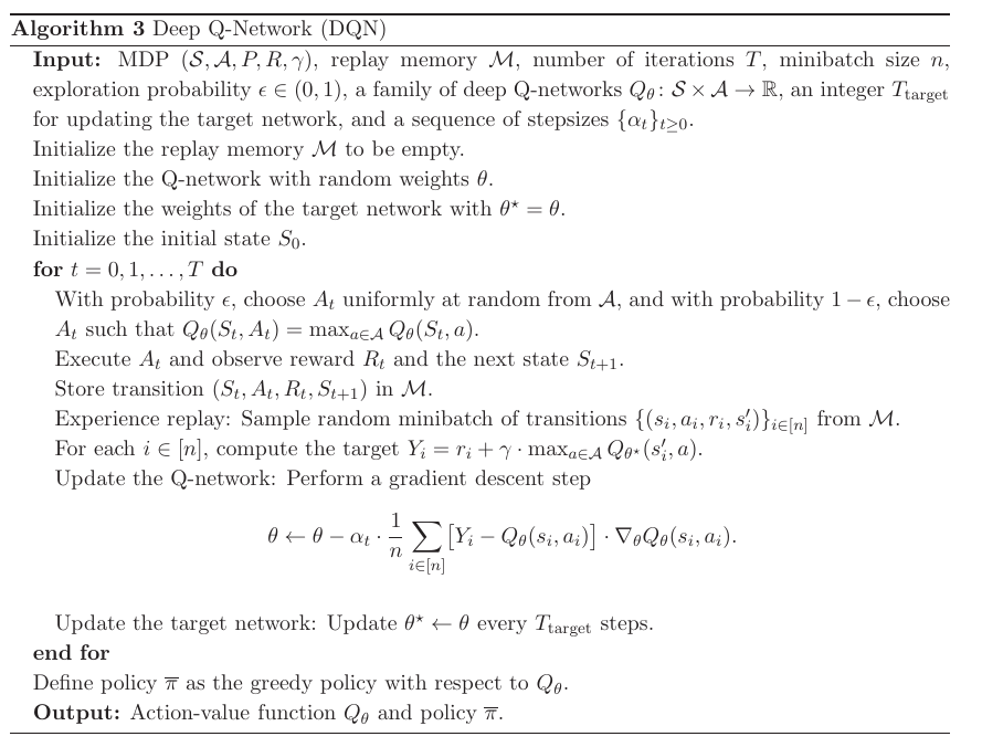
[Source: *Fan, Jianqing, et al. "[A theoretical analysis of deep Q-learning](https://arxiv.org/abs/1901.00137)." Learning for Dynamics and Control. PMLR, 2020.*]
## 5 Double DQN
The issue: **Overestimation bias**
The estimated Q-function, denoted $ Q_t $, is noisy (has variance). We have
$$\frac{1}{m} \sum_a(Q_t(s,a) - V^*(s))^2 = C$$
for some $ C>0 $, where $ m $ is the number of actions, $ V^*(s) $ is the optimal V-function. This leads to
$$\underset{a}\max Q_t(s,a) \geq V^*(s) + \sqrt\frac{C}{m-1}$$
(full proof see *Appendix* of *[Deep Reinforcement Learning with Double Q-learning](https://arxiv.org/abs/1509.06461)*)
Recall $ V^*(s) = \underset{a'}\max Q^*(s,a') $, we have
$$\underset{a}\max Q_t(s,a) \geq \underset{a'}\max Q^*(s,a') + \sqrt\frac{C}{m-1}$$
i.e. the max of Q-estimation is biased upward. Recall that this maximization is used in the Q-target, which the Q-function is trained to approximate:
$$y = R(s,a) + \gamma \underset{a}\max Q_t(s',a)$$
As training proceeds, this overestimation propagates, so the learned Q-function tends to remain overestimated compared to the true value. This is also shown experimentally below:
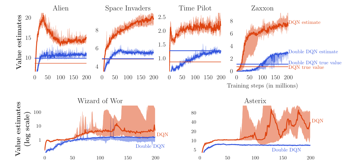
[Source: *Van Hasselt, Hado, Arthur Guez, and David Silver. "[Deep reinforcement learning with double q-learning](https://arxiv.org/abs/1509.06461)." Proceedings of the AAAI conference on artificial intelligence. Vol. 30. No. 1. 2016.*]
The solution: **Decoupling action selection and evaluation**
In naive DQN, the same network $ \theta' $ is used to obtain the action with max Q-value, and evaluate the corresponding Q-value.
In Double DQN, we use different networks to choose the best action and evaluate it. Specifically, the online Q-network $ \theta $ is used to select the action, and the target network $ \theta' $ is used to evaluate it.
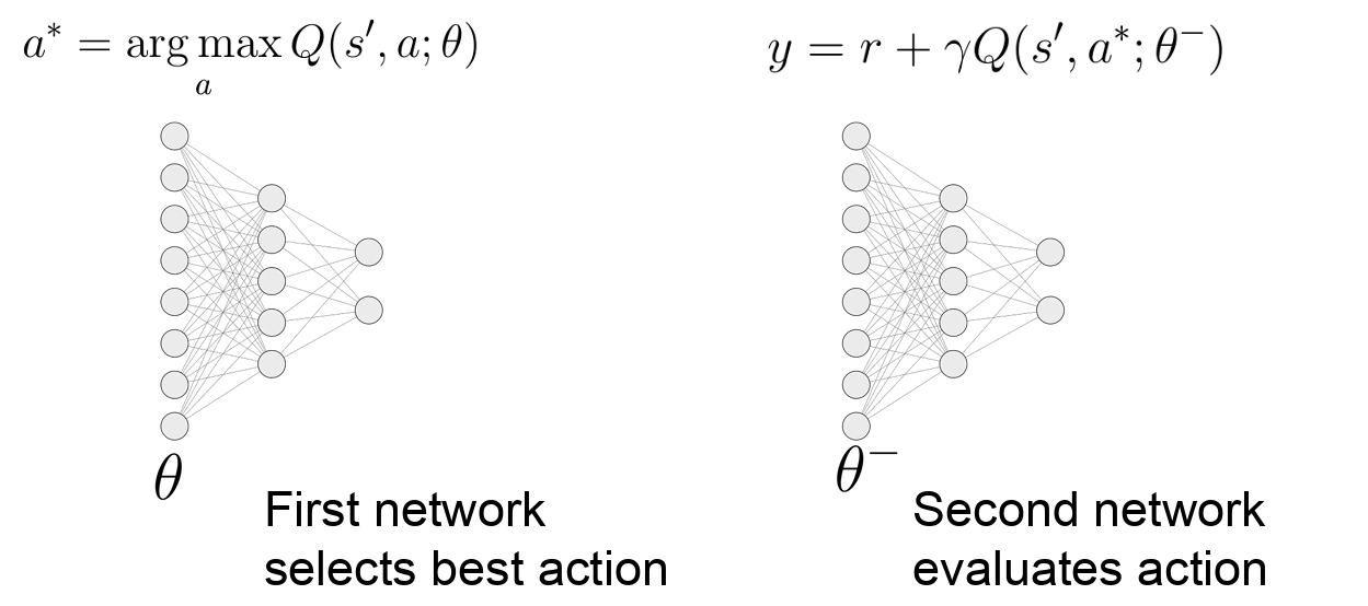
[Source: [Cornell *CS 4782 Deep Learning* Lecture Slides, Week 8: Deep Q-Learning](https://www.cs.cornell.edu/courses/cs4782/2026sp/slides/in-class/inclass21.pdf)]
This can reduce the overestimation in Q-value. In the naive DQN,
$$y_{naive} = R(s,a) + \gamma \underset{a}\max Q(s',a;\theta')$$
In double DQN,
$$y_{Double} = R(s,a) + \gamma Q(s',a^*;\theta')$$
Regardless of $ a^* $, we must have
$$Q(s',a^*;\theta') \leq \underset{a}\max Q(s',a;\theta')$$
So $ y_{Double} \leq y_{naive} $. We see that in Double DQN, Q is optimized to match a target with reduced upward bias, alleviating the overestimation issue.
## 6 Summary
- It's tricky to model the environment, disincentivizing model-based approaches like value iteration.
- Model-free approaches like Q-Learning use experience to learn, leveraging $ \epsilon $-greedy policies to encourage exploration.
- For large or continuous state spaces, we cannot feasibly store all the Q-values so we use a DQN instead.
- Naively training on sequential transitions violates the iid assumption, so we store transitions in an experience replay and sample minibatches.
- The Q-target depends on the same parameters that it updates, creating a moving target; a frozen target network stabilizes training by fixing the target for $ T $ steps.
- Double DQN alleviates the overestimation bias by decoupling action selection and evaluation.
## 7 References
- [Cornell *CS 4782 Deep Learning* Lecture Slides, Week 8: Deep Q-Learning](https://www.cs.cornell.edu/courses/cs4782/2026sp/slides/in-class/inclass21.pdf)
- Fan, Jianqing, et al. *"[A theoretical analysis of deep Q-learning](https://arxiv.org/abs/1901.00137)." Learning for Dynamics and Control.* PMLR, 2020.
- Van Hasselt, Hado, Arthur Guez, and David Silver. *"[Deep reinforcement learning with double q-learning](https://arxiv.org/abs/1509.06461)." Proceedings of the AAAI conference on artificial intelligence.* Vol. 30. No. 1. 2016.